|
|
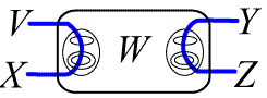
| an n-adic spot with a LI attached to each of its n hooks, the entire complex in the same area, and none of the LI' s having any other connections or branchings is a beta graph; this graph has n "loose ends." |
WE now move to a close-up study of the beta part of the graphs. As we have seen, alpha may be considered to be a system of propositional calculus; to be sure, alpha's approach to truth-functional logic differs from approaches utilizing more ordinary notation, but it is relatively easy to grasp intuitively. We may even react quite favorably, in fact, to features of alpha like the symmetry -- or irrelevancy of position -- and associativity of conjunction implicit in the "simultaneous unseparated occurrence" of alpha graphs, this in spite of the complexities introduced by such features in, say, the translation of the graphs into ordinary notation and vice-versa. Beta, however, is a kettle of fish taken from somewhat deeper waters. Beta, we shall find, bears a relation to alpha similar to that borne by the ordinary first-order predicate calculus to the ordinary CPC. But as was indicated in the Introduction, the "individual variable" and the method of quantification in beta are, apparently, radically different from the corresponding elements in the ordinary predicate calculus. While intuition may give willing assent to the characteristic features of alpha, it is possible that it may be a bit more hesitant about beta. But a careful examination of beta should lead to a more willing acceptance of its features; such an examination will be the aim of this chapter.
The project of chapter I was a comparison of the alpha system with the ordinary CPC. As we might infer from the remarks we have just made, the project for beta will involve a comparison of beta with ordinary classical predicate calculus. We shall, in fact, compare beta with the complete classical first-order calculus with identity.
The notation of beta is -- as we have already seen -- considerably more complicated than that of alpha. We shall, then, first set down some remarks on that notation. much of the terminology of the beta system will be explained, and a list of rules characterizing the beta graphs will be set down.
In our comparison of alpha with the CPC, we found it convenient to use two formulations of the CPC. Similarly, we shall here employ two formulations of the first-order calculus with identity. The first, Fr, will -- like Pr of chapter I -- have conjunction and negation as primitive operators; the other, Fw, will use implication and constant false proposition, as did Pw. Both systems will have the universal quantifier and the sign of identity as primitive. Fr and Fw are both full classical first-order calculi with identity, and are "equivalent" to each other in the sense that Pr and Pw are equivalent.
We shall provide a set of instructions, which shall be called the (one-one) function f¢, and which -- when applied to any beta graph X as argument -- will "translate" it into a unique closed wff -- called f¢(X) -- of the logic Fr.
We shall also provide a set of instructions, to be called the (one-one} function g¢, which -- when applied to any closed wff A of the logic Fw -- will translate it into a unique beta-graph -- to be called, in this case, g¢(A).
The description of the functions f¢ and g¢ will parallel in many ways the description of the functions f and g of chapter I, Then will come an investigation of "theorem generation" in beta. This will involve an explicit statement of the rules of transformation, or inference, in beta. Here we shall show both that beta is a logic and that it is consistent.
The next step will be a proof -- through a series of lemmas showing that the beta rules of transformation have analogs in Fr -- that:
If a beta graph X is a theorem of beta, then the closed wff f¢(X) is a theorem of Fr.
The proof of the converse of this metatheorem, however, does not follow as easily as it did in alpha, and will be taken up later in this chapter.
Then we shall achieve a most remarkable result. We shall show that
A closed wff A is a theorem of the logic Fw iff the graph g¢ (A) is a beta theorem.
In the process we will give what amounts to a set of semantical rules for beta, that is, a means of assigning an interpretation to any beta graph. This will enable us to say what it means for a beta graph to be valid.
We may then enter the final phase of our beta project. This will be to prove that every valid beta graph is a theorem of beta. This is. in effect, to prove that beta is complete.
Once this is done, it will follow that:
If the closed wff f¢(X) is a theorem of Fr, then X is a theorem of beta.
We shall thus have established that the set of beta theorems maps one-one into the set of theorems of the first order calculus with identity, and more importantly, that the set of theorems of the first-order calculus with identity map into the set of beta theorems. Given the natures of the mapping functions, f¢ and g¢, we will then have shown beta itself to be a complete first order calculus with identity, and to have a recursively unsolvable decision problem.
2.1 The Set of Beta Graphs
In the Introduction we examined the beta system -- at arm's length -- and got some idea of what it is for a sign-complex to be a beta graph. In this section we shall look more closely at the set of beta graphs. Our purpose shall be two-fold; we wish:
|
(1) |
To recursively characterize the set of beta graphs, and in the process to say what it means for two beta graphs to be identical, and | |
|
(2) |
To lay the groundwork for the definition of the functions which will translate beta into an ordinary logic and vice-versa.. |
The characterization of the set of alpha graphs offered us no problem at all. Given the set of minimal alpha graphs and the "operations" S(X) and J(X1, . . ., Xn), we were easily able to characterize the set of alpha graphs.
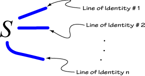
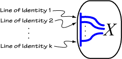
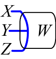
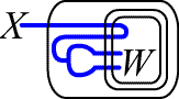
As might be gathered from the Introduction, beta will be more difficult to handle than was alpha. It is fairly evident that beta, with its 'spots," is a "calculus of predicates." And among the signs of beta is that protean "line of identity" (which we shall often abbreviate as "LI"); this sign is sometimes itself a graph -- and then has a propositional interpretation -- and sometimes, as we remarked in the Introduction, a kind of "bound variable." The presence of the LI in the vocabulary of beta considerably complicates both the characterization of the set of beta graphs and the definition of "translation functions" paralleling alpha's f and g.
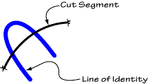
Let us now define a term we shall find quite useful in our treatment of beta. We shall call a LI "geodesic" between two points on the SA iff it connects those points, crossing only the cuts which may be between them, and each of those cuts only once.
We shall now provide a set of rules which will characterize the set of beta graphs. These rules might also be considered rules for the "generation" of any beta graph [they are, effectively, "rules of formation" which enable us to identify legal beta graphs].
| 2.1i | The "null-graph," b, is a beta graph. | |||
| 2.1ii | ' |
|||
| 2.1iii | ' |
|||
| 2.1iv |
|
|||
| 2.1v | Where X is a beta graph and has n loose ends, S(X) is a beta graph and has n loose ends. | |||
| 2.1vi | Where X1, . . ., Xn, n ³ 2, are n beta graphs admitted by rules 2.1ii-2.1v above, and the total number of loose ends in these n graphs is m, then J( X1, . . ., Xn) is a beta graph and has m "loose ends." | |||
| 2.1vii | Where X is a beta graph having n loose ends, and X¢ is like X except for having two of those ends connected by a geodesic LI, then X is also a beta graph, and has n - 2 loose ends. |
It should be fairly clear that these rules will admit all and only the sign complexes which Peirce would consider beta graphs. Two beta graphs are identical iff they have identical "histories of generation" by the above rules.
It is evident that for the generation of a given beta graph by these rules, the insertion by rules 2.1ii-2.1iv of certain signs involving LI 's is essential to the generation of that graph. To put it another way, we may say that for the description of the "LI network" of a given graph, it is necessary that we know the locations in that graph of certain. "critical points" in that network. These "critical points" are:
|
(1) |
The places where LI 's connect to hooks of spots, | |
|
(2) |
Branchings in LI' s, | |
| (3) | The places where LI's come to "dead ends," | |
| (4) | The places where LI's become "non-geodesic." |
In the "generation" of a beta graph by rules 2.1i-2.1vii, these are the points which must "get into" the graph through rules 2.1ii-2.1iv, The remainder of the LI network of the graph may be "filled in" by rule 2.1vii.
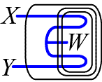
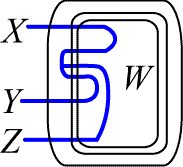
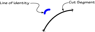
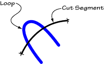
A comment on (4) above may be in order. If a LI is non-geodesic between two points, a little thought will tell us that there is at least one place along its length where it crosses a cut and then re-crosses the same cut thus:
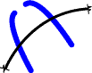
Such LI formations will be called "loops." Consider any non-geodesic LI, snaking its way through a beta graph. If this LI were to be broken at all its loops, like this:

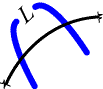
it is obvious that each of the LI's resulting from such breaking would be geodesic. If we wish to picture to ourselves the "generation" of a beta graph containing non-geodesic LI's (which is the same as saying, "Containing loops"),, we may imagine that LI's with two "dead ends" are first inserted by rule 2.1ii at places in the graph where loops will eventually appear; the connections which will then "create" the loops may be made by 2.1vii. So justified by 2.1ii we have
And then justified by 2.1vii:
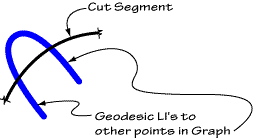
The other three kinds of critical point in the LI network require, I think no further explanation. We shall see that these "critical points" play an important role in the translation of beta into an ordinary logical system in such a manner that X and Y translate as the same formula in ordinary logic iff the graphs X and Y are identical, that is, have the same "history of generation."
We will here note one special but unimportant kind of LI formation; if a LI "twists back on itself" and joins end to end, all in the same area, to form the graph:
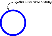
(This is not a cut, but a LI) with no branchings and homeomorphic to a circle, that LI we shall call the "cyclic graph."
We may also add, as a bit of nomenclature, that we shall say that a LI "terminates" when and only when either it comes to a dead end, connecting to nothing, or it joins two other LI's at a branching.
2.2 The Beta Graphs and the WFFS of Classical Predicate Calculi
2.21 The Systems Fr and Fw
As was the case in Section 1.2 of our investigation of alpha, we shall set out two systems of classical logic; in this case these will be systems of first-order predicate calculus with identity. The systems themselves will be celled Fr and Fw; we shall be interested in a particular subset of the set of wffs of each of these systems, the set of closed wffs (for closed wff we shall write "cwff") . The sets of cwff' s of Fr and Fw respectively will be (Fr) and (Fw) , and we shall specify what it is to be a cwff.
We shall employ the upper-case letters at the beginning of the Western
alphabet [or l.c. Greek letters] as metalinguistic variables for wffs and for predicates, and the
lower-case letters at the beginning of the Western alphabet as variables for
individual variables. The letters 'x', 'y', . . ., will, as usual,
be the individual variables themselves. An upper case letter will normally
represent a predicate only when it is followed by a sequence of lowercase
letters, which will represent or be the arguments of that predicate. "![]() r
A" shall mean "the closure of A is a theorem of Fr"
and "
r
A" shall mean "the closure of A is a theorem of Fr"
and "![]() w A"
shall mean "the closure of A is a theorem of Fw" The
notion of closure is as in the revised edition of
Quine's Mathematical Logic.
w A"
shall mean "the closure of A is a theorem of Fw" The
notion of closure is as in the revised edition of
Quine's Mathematical Logic.
The primitive signs of the system Fr are: A denumerable infinity of signs, w, x, y, z, w1, x1, . . . , called the "individual variables," the signs '(', ')', '
~' as in Pr, the sign ' =', a constant dyadic predicate called "the sign of identity."The rest of the signs of Fr are "variable predicate symbols," which we need not show, and each of which has associated with it a natural number
³ 1 called its "degree."The primitive signs of Fw are: individual variables and variable predicate symbols as in Fr, the signs 'C' and '
Æ' as in Pw, the sign 'I ', a constant dyadic predicate called "the sign of identity," and the sign 'P' called the "sign of the universal quantifier."Again, we shall assume all the standard definitions, including that of the existential quantifier. Note that the kind of notation used in practice is frequently a matter of convenience. It will be recalled that sometimes in our work with Pr in chapter I we used the Polish notation, even though the primitive symbols of that system are not in that notation. We did this because we feel that the Polish notation is superior to the "PM-type" notation for work in the PC. For extended work in quantificational systems, however, we prefer the "PM-type" notation; hence, we shall often, in this chapter, write out Fw formulas in that notation. It is always to be understood, however, that a formula so presented is a definitional "abbreviation" of a formula in primitive notation.
Now, the rules of formation for Fr are:
| 2.21i |
|
|
| 2.21ii |
|
|
| 2.21iii |
|
|
| 2.21iv |
|
|
| 2.21v |
|
An occurrence of a variable a is called "bound in a wff A" if
it is in a wf part of A of form
![]() (a)B
(a)B![]() .
Otherwise it is called "free in A." A wff in which no variable has a free
occurrence is called "closed." We write "cwff" for "closed well-formed-formula."
.
Otherwise it is called "free in A." A wff in which no variable has a free
occurrence is called "closed." We write "cwff" for "closed well-formed-formula."
The rules of formation for Fw are:
| 2.21vi | Æ is wf | |
| 2.21vii |
|
|
| 2.21viii | This rule is the same as 2.21ii. | |
| 2.21ix |
|
|
| 2.21x |
|
The remarks concerning "freedom," "binding," etc. for Fw apply here as well, mutatis mutandis.
As axioms for both systems we shall employ versions appropriate to the respective primitive notations of Quine's "axioms of quantification," *100, *101, *102, and *103. In addition we shall have the following axiom schemata for Fr:
|
|
||
|
|
In Fw the extra axiom schemata are:
|
|
||
|
|
The rule of inference for each system shall be an appropriate version of Quire's *104. All of Quine's metatheorems referred to here are, of course, from the revised edition of Mathematical Logic.
2.22 The Translation Function f
¢In chapter I we showed how two functions, f and g, might be defined. The former was a function which translated alpha graphs into formulas of an ordinary PC, and the latter translated formulas of an ordinary PC into alpha graphs. We are now prepared to present the similar "translation functions" for the beta system. These functions will relate beta to the calculi Fr and Fw, and will be called f¢ and g¢ respectively.
We shall first consider the function f¢. This function takes as arguments the members of the set of beta graphs, and finds its range in the set (Fr) of cwffs of Fr. For the purposes of translation, we shall add to the vocabulary of beta (temporarily) a "translation vocabulary" consisting of three spots.
|
(1) |
A unary spot, Q, | |
|
(2) |
A binary spot., L, | |
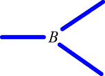
| (3) | A ternary spot, B. |
We now apply the function f¢ to an arbitrary beta graph X. Given X, attach an instance of the spot Q to each dead end of a LI occurring in n X.
Next, we will recall from our earlier remarks what a loop is. Wherever a loop occurs in X,
break it like this
and then attach the two LI ends thus freed, one to each hook of the spot L:
And then, there may be branchings in X. Each of them will look like this:
Erase the center of the branching thus:
and attach each of the loose ends of LI's thus formed to one of the hooks of the spot B, like this:
There may be "cyclic graphs" occurring in X. Wherever such a graph occurs, erase it and write the sign-complex '(
$w)(w = w)'. Consider this sign-complex for the moment as if it were a graph.It is now clear that all the LI's remaining in the graph X are, must be, geodesic. Effective means are certainly available for ordering the set of LI's remaining in X (we remark in passing that there are now, of course, no dead ends or branchings left in X). Order this set, and then associate with each such LI a distinct individual variable of the system Fr (excluding 'w' ). If a given LI in the graph as it now stands is associated with the variable a, erase that LI and write the variable a at the points in the graph which were connected by the LI in question; that is, attach a to the hooks to which the LI had been connected. Do this for all LI's remaining in the graph. Where X was the original graph, call the version as so far transformed "X
¢."X¢ is a graph free of LI's. Where X used LI ' s to identify arguments of spots of various kinds, X¢ uses individual variables. In this it is much closer to a formula of ordinary logic than was X. It is also much more similar to an alpha graph. In fact, we may now use an appropriately altered version of the function f of chapter I to convert X¢ to a unique wff of Fr. If the cyclic graph occurred in the original graph X, let the wff '(
$w)(w = w)' be carried over into the formula we are forming unchanged. The spots Q, L, and B should be associated with constant predicates Q, L, and B of Fr, the predicates being unary, binary, and ternary respectively. All individual variables should be carried over from X¢ as arguments of the predicates associated with the spots to which those individual variables were attached in X¢; let the arguments of each of the predicates L and B be ordered alphabetically. Let each of the variable spots in X¢ be associated with an appropriate variable predicate symbol in the formula being formed from X¢. Now assign quantifiers to the variables of this formula. Begin with the alphabetically lowest variable which appears free in the formula. Where this variable is a, write the quantifierNow for each variable a, wherever
![]() Qa
Qa![]() occurs, replace the
occurs, replace the ![]() Qa
Qa![]() by
by ![]() a = a
a = a![]() .
For each a and b, wherever
.
For each a and b, wherever
![]() Lab
Lab![]() occurs, replace it by
occurs, replace it by ![]() a
= b
a
= b![]() . For each a,
b, and c, wherever
. For each a,
b, and c, wherever
![]() Babc
Babc![]() occurs, replace it by the formula
occurs, replace it by the formula
![]() (
(
This completes the instruction for f
¢ , Where the graph we started out with was X, the cwff of Fr we now have i s f¢ (X). This formula is the unique translation by the function f¢ of the graph X into the logic Fr.2.23 The Translation Function g
¢The function g of chapter I translates the CPC Pw into the alpha system. The function g¢ will perform a similar function for the first-order calculus and the beta system. Consider an arbitrary member of the set (Fw), A. A is a cwff; its signs may consist of individual variables, predicate signs of various degrees, the sign of identity, 'I', the sign of implication, 'C', the constant false proposition, '
Æ', and the sign of universal quantification, 'P '. Now in the Fw wff A, let us for the time being consider the sign complexesNow we have transformed A, through A¢ ,
into a graph, but one without lines of identity. Turn next to the subformulas
![]() Iab
Iab![]() ,
in that graph. Replace the formula
,
in that graph. Replace the formula
![]() Iab
Iab![]() with the graph
with the graph
for each such formula. The motivation behind this move is easy to understand.
If we had taken the fairly obvious step of simply replacing
![]() Iab
Iab![]() by the graph
by the graph ![]() , we would have no
means of distinguishing the translation of
, we would have no
means of distinguishing the translation of
![]() Iab
Iab![]() from that of
from that of ![]() Iba
Iba![]() -- for
-- for ![]() and
and
![]() are, in the beta system,
identical graphs; beta does not distinguish left-from right or up from down. The
arrangement of cuts in
are, in the beta system,
identical graphs; beta does not distinguish left-from right or up from down. The
arrangement of cuts in
however, distinguishes it from
and enables us to offer distinct translations for
![]() Iab
Iab![]() and
and ![]() Iba
Iba![]() (n1).
(n1).
Now turn to the formulas
![]()
But if n
¹ 0, replace the appropriate
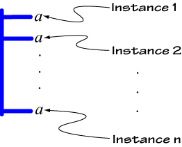
That is, replace it with a LI having n branchings, at the end of each of
which is the variable a (the "Instance ..." labels in the above diagram are, of
course, not part of the sign-complex replacing
![]() Pa
Pa![]() ).
).
Now we are ready to complete our translation of the original formula A into a beta graph. In essence, what we are about to do is just the reverse of a step we took in our description of the function f¢ --there we replaced geodesic LI's with individual variables, and here we will replace individual variables with geodesic LI's. So go to one of the complexes
standing in our graph. This sign-complex corresponds to a quantifier in the original cwff A, which quantifier binds n occurrences of the variable a in A. There are, in our graph as it now stands, n points -- each marked by the variable a--which points correspond to the n occurrences of a in A bound by the quantifier in question. Let each of the branchings in the above pictured complex be connected by a geodesic LI to one of these points; erase each of the a's as the LI's are drawn (these variables are no longer needed as place holders once the LI's are present). These connections should be made in some effectively determined order; that is, we should have a mechanical procedure for telling which branch of the pictured sign-complex is to be attached to which point in the graph -- we will not describe such a procedure, but it should be clear that it would be quite easy (if irrelevantly tedious) to do so.
The above procedure of replacing variables by LI's should be continued until all variables in the graph have been replaced by LI's. What we have when we are finished is a beta graph with its variables replaced by LI's, and with distinctive signs involving LI's replacing quantifiers and identity formulas. Where A was the original Fw cwff , the graph we now have is g¢(A).(n1)
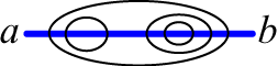
We must draw attention here to the fact that g¢ as described above is not, strictly speaking, one-one, but many-one. This is so because if B is a mere alphabetic variant of the cwff A, then with the procedure we have outlined, g¢((B) will be precisely the same graph as g¢(A). As a simple example, the Fw cwffs '
PxIxx' and 'PyIyy' will both translate as the beta graph
One might comment that this is not a serious difficulty; from one point of view, you might even consider that if A and B are merely alphabetic variants of each other, then they are essentially the same formula -- from this point of view, g¢ as it stands would already be one-one. But I submit that there are many possible ways of making g¢ take account of alphabetic variance, to yield distinct graphs as values for of cwffs s A and B when A and B are distinct alphabetic variants of each other. Again, however, the description of such means has a definite tendency to be tedious -- to be a kind of intellectual nitpicking. And it adds little to the main thrust of this paper. Hence, let us state simply that provisions may be built into g¢ to take care of alphabetic variance. Once this is accounted for and our explicit description of g¢ taken as above presented, we may assert that g¢ is a one-one recursive word function.
It will be recalled from chapter I that the function g mapped
(Pw) onto a
recursively characterizable subset of the set of alpha
graphs, ![]() a.
From the description we have given of g¢
, it is clear that the beta graphs constituting the range of g¢
are members of a set in many ways similar to
a.
From the description we have given of g¢
, it is clear that the beta graphs constituting the range of g¢
are members of a set in many ways similar to
![]() a
. As we shall see later in this chapter, this set too is recursive, although its
characterization is a bit more complex than that of
a
. As we shall see later in this chapter, this set too is recursive, although its
characterization is a bit more complex than that of
![]() a.
a.
The set of beta graphs which is the range of g¢
we will call ![]()
2.3 Beta as a Logic
2.31 Theorem Generation in Beta
We now move from the study of the set of objects which qualify to be called beta graphs to the study of the subset of that set which is characteristic of beta as a logic -- the theorems of beta. We have remarked that every beta graph is to be considered a closed quantificational formula. It follows rather trivially from this that every theorem of beta will be a closed formula. This fact is not as restrictive as it might seem at first; it is true that there are formulations of the predicate calculus which recognize some open formulas as theorems, but this is by no means necessary. The system of Quine' s Mathematical Logic, for example, is one in which every theorem is a cwff ; we have, in fact, based our systems Fr and Fw upon the "quantification theory" of Mathematical Logic.
Beta as a logic is built upon alpha; this becomes apparent in an examination of the set of rules for beta given in 4.505-508, for example. This means that the six rules of inference for alpha are to be considered to apply to beta graphs as well, insofar as the transformations wrought by these rules do not affect the LI ' s of a graph; in addition, the logic beta will contain what we may call extensions of these rules for cases involving transformations affecting LI ' s; we shall discuss this presently.
We will recall that the single axiom for alpha is the simple null-graph b. As we noted in the Introduction, Peirce indicates that another graph is to be what we would call an axiom for beta (4.567). For our purposes, we may take this graph to be the doubly terminating LI -- the LI with two dead ends -- standing alone on SA, with no branchings or connections. It is evident that given this graph as axiom and the rule Rers, b may be derived as a theorem of beta. Let us then say that the double-dead-end LI standing on SA is the only axiom of beta.
In beta we have, as we have mentioned, the six alpha rules of transfomation. In this sense beta is founded upon alpha just as quantification theory is founded upon the PC. There are also certain specific beta extensions of these rules which we shall now list (Cf. 4.505-508). Note that we use the same notation for these rules as we did for the alpha rules; the conditions we list here are to be considered clauses extending the alpha conditions for the respective rules of transformation. Following, then, are the "extending clauses" for the rules of transformation as they shall be employed in beta:
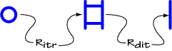
| Rins(Y, X): | Is true provided Y is exactly like X except that in an oddly enclosed area where X has two LI dead end termini, Y has not those two termini but a continuous LI joining the points in n Y corresponding to the points in X to which the terminating LI's were connected (this rule, in other words, permits the joining of two "loose ends" in an oddly enclosed area). | |||||||||||
| Ritr(Y, X): |
|
|||||||||||
| Rbcl(Y, X): | Is true as provided in chapter I for the alpha system, and in addition, it is true if the two cuts of the biclosure present in Y but not in X intersect LI's in such a manner that the intersected segments of LI ' s pass from entirely outside the outer to entirely inside the inner cut -- no branching, loops, dead ends, or any other kind of graph is permitted in the annular space between the two cuts of the biclosure. The only signs that may be there are the LI ' s enroute from outside to inside the biclosure. | |||||||||||
| Rers(Y, X): | Is true iff Rins(S(X), S(Y)) is true. | |||||||||||
| Rdit(Y, X): | Is true iff Ritr(X, Y) is true. | |||||||||||
| Rnbc(Y, X): | Is true iff Rbcl(X, Y) is true. | |||||||||||
Thus do we state, for the purposes of this chapter, the beta versions of the rules of transformation, which in the Introduction were numbered 0.07 to 0.12. As is evident, these rules are not easy to express in English (or French, German, or Sanskrit, for that matter); but notwithstanding the complexity of their statement, they are intuitively not at all difficult to grasp.
At this point it might be a good idea to review the examples of the applications of these rules which are presented in the Introduction.
We may now move to the statement of a metatheorem which parallels *1.01 in the alpha chapter:
| *2.01 | Beta is a logic. |
PROOF: Immediate from our definition of "logic" and the above statements
regarding the axiom and rules of inference of beta.![]()
Alonzo Church(n1) makes use of the notion of the "associated form of the propositional calculus" -- abbreviated "afp" -- in order to show that a first-order predicate calculus which he presents is consistent. We here introduce an analogous notion for the beta system; we shall speak of "the associated form of the alpha system" or "afa" of a given beta graph. It is clear that the spots of beta may be correlated one-one with the members of the set Ma (aside from b), the minimal graphs of alpha. Perform such a correlation, and for any beta graph X, replace each spot of X with its associated minimal graph of alpha; in the process, erase the entire LI network of X. The result of applying these instructions to a beta graph X is an alpha graph, and this graph will be called the afa of X.
| *2.02 | If X is a theorem of beta, then the afa of X is a theorem of alpha. |
PROOF: The introduction of any spot with its
connected LI ' s -- the initial introduction -- into a beta graph is exactly
like the initial introduction of an alpha minimal graph in the proof of
an alpha graph in that that introduction requires an
application of Rins. Furthermore, all the beta rules of
inference as they apply to transformations involving spots and cuts are directly
parallel to the alpha rules of transformation, prescinding from the effect these
beta rules may have upon any LI 's present. If, then, there is a proof for the
beta graph X, then there is a proof in alpha directly paralleling the
proof of X; where the proof of X performs some transformation
involving a spot, the proof in alpha performs an analogous transformation
involving an alpha minimal graph associated with the spot in question. The proof
in alpha has no steps paralleling those in beta which affect only LI's, but this
makes no difference, as these steps do not affect the location, etc., of the
spots in X. But if such a proof exists in alpha, it is, by the definition
of afa, a proof of the afa of X. Thus if X is a beta theorem, the
afa of X is an alpha theorem.![]()
| *2.03 | Beta is consistent. |
PROOF: It is clear that not every beta
graph has an afa which is a theorem of alpha -- an arbitrary spot with its LI '
s at its hooks, the whole complex standing alone on SA is an example of such a
graph. But by *2.02 through modus tollens, then, there are beta
graphs which are not theorems of beta, and beta is consistent.![]()
2.32 The Logic Beta in the System Fr
In section 2.22 we defined a function f¢ which maps the set of beta graphs into the set of cwffs of Fr. Our project now is to show that whenever X is a theorem of beta, f¢(X) is a theorem of Fr. We state first the following lemma:
| LEMMA 2.04 | Where X is the axiom of beta, f¢(X) is a theorem of Fr . |
PROOF: The axiom of beta is a simple
double-dead-end LI standing alone on SA. Then, by the definition of f¢, f¢(X)
is the cwff
![]() (
(
This lemma shows that the axiom of beta is correlated by f¢ to a theorem of Fr. We now move to lemmas concerning the beta rules of inference; so far as the "alpha clauses" of these rules are concerned, we know by our work in chapter I that they "hold" in Fr, since Fr is, essentially, "based on" the CPC Pr.
| LEMMA 2.05 |
Whenever, for beta graphs X and Y, Rins(Y,
X) is true, then if
|
| LEMMA 2.06 |
Whenever, for beta graphs X and Y, Rers(Y,
X) is true, then if
|
PROOF: (As we will recall, ''![]() r
r
![]() A
A![]() "
is to be read, "The closure of A is a theorem of Fr."
) Based on our work in chapter I (lemmas 1.03 and 1.04) we may
take it as fairly evident that the following hold:
"
is to be read, "The closure of A is a theorem of Fr."
) Based on our work in chapter I (lemmas 1.03 and 1.04) we may
take it as fairly evident that the following hold:
|
If
|
(1) | |
|
If
|
(2) |
Now let us take as hypotheses:
| Hyp. | For beta graphs X and Y, Rins(Y, X) is true | (3) |
| Hyp. |
|
(4) |
Now let us define as "Pren(A)" some specific prenex-normal form of the cwff A; we then have:
| (4), Df. Pren(A) |
|
(5) |
By (3) and the definition of Rins, there are, in an oddly
enclosed area of the graph X two "loose ends" of LI ' s, which loose ends
are connected in the graph Y, Hence, by the definition of the function f¢,
Pren(f¢(X))
may be represented by the schema
![]() PA(a
= a.b = b)
PA(a
= a.b = b)![]() ,
where
,
where ![]() a
= a
a
= a![]() and
and ![]() b
= b
b
= b![]() are associated respectively through f¢
with the two loose ends in question. It should be clear that we have replaced f¢(X)
by one of its prenex normal forms to get any quantifiers which may have been
introduced by f¢ out of
the way. But now, since
are associated respectively through f¢
with the two loose ends in question. It should be clear that we have replaced f¢(X)
by one of its prenex normal forms to get any quantifiers which may have been
introduced by f¢ out of
the way. But now, since
![]() PA(a
= a.b = b)
PA(a
= a.b = b)![]() is the same formula as Pren(f¢(X)),
we have by (5) above:
is the same formula as Pren(f¢(X)),
we have by (5) above:
|
|
(6) |
But by the laws of Fr, it is trivially true that
|
|
(7) |
Then, by (1), (6), (7):
|
|
(8) |
By Df. Rins, the graph Y differs from the graph X
only in having the two "loose ends" in question. connected; the "individuals"
represented by these two "loose ends" in X are then identified in Y.
Step (8) shows that the same identification may be accomplished in the
system Fr. There should be no trouble in seeing, given the
definition of f¢ and Rins
and the substitutivity of identity, that
![]() PA(a
= b)
PA(a
= b)![]() is a prenex normal form such that:
is a prenex normal form such that:
|
|
(9) |
Then, by (8), (9)
|
|
(10) |
This proves the first of the two lemmas involved. The
relation of the second of these lemmas to the first is fairly clear, and
once the first has been proven, the proof of the second should offer no
difficulty.![]()
We now turn to two more lemmas:
| LEMMA 2.07 |
Whenever, for beta graphs X and Y, Ritr(Y,
X) is true, then if
|
| LEMMA 2.08 |
Whenever, for beta graphs X and Y, Rdit(Y,
X) is true, then if
|
PROOF: Recall that for. Ritr (and Rdit is just the converse of Ritr) there are four basic cases to be considered:
| 1. | When X is transformed into Y by the extension of a branch from a LI. |
| 2. | When X is transformed into Y by the extension inwards of the loose end of a LI. |
| 3. | When X is transformed into Y by the iteration of a subgraph Z (defined by the notion of the "boundary" of a subgraph) in the same area or inwards. |
| 4. | When X is transformed into Y by an iteration as in 3, with the maintenance of certain LI connections. |
(For details, see the original statements of the definitions of Ritr and Rdit earlier in this chapter.)
For all of these cases, the following hypotheses will hold:
| Hyp. | For beta graphs X and Y, Rity(Y, X) is true | (1) |
| Hyp. |
|
(2) |
Now let us consider the first case. Here Y differs from X only in having, at some point, a branch (with loose end) extending from an LI where X has no such branch. Let a be the variable in f¢(X) associated with the LI involved (that from which the branching is to be extended). The cwff f¢(X) will then contain at some point a subformula, a function of a containing all occurrences in f¢(Y) of a, Aa. The cwff f¢(Y) contains a similar subformula in conjunction with a formula which by f¢ represents a branching with a loose end. By f¢, the conjunction occurring in f¢(Y) in place of Aa will be of general form
|
|
(3), |
where the three formulas involving 'w' represent the branching itself,
and ![]() c = c
c = c![]() represents the new "loose end" itself. But clearly, in Fr,
represents the new "loose end" itself. But clearly, in Fr,
|
|
(4). |
Then, since f¢(Y) differs from f¢(X) only in having the equivalent of (3) where f¢(X) has the simple Aa, by the substitutivity of the biconditional, (2), and (4) we have
|
|
(5). |
We now consider the second case. Here Y differs from X only in
having the loose end of a LI "extended geodesically" inwards from the original
position it occupied in X. This means, by Df.f¢,
that somewhere in f¢(X)
there will be a subformula ![]() a
= a
a
= a![]() corresponding to the
loose end in X and the scope of and bound by a quantifier
corresponding to the
loose end in X and the scope of and bound by a quantifier
![]() ($a)
($a)![]() ,
and that in f¢(Y)
that formula
,
and that in f¢(Y)
that formula ![]() a = a
a = a![]() will not be. where it was in f¢(X)
but will be elsewhere in the whole formula, though still in the scope of and
bound by that same quantifier (we know from Df. f¢
that
will not be. where it was in f¢(X)
but will be elsewhere in the whole formula, though still in the scope of and
bound by that same quantifier (we know from Df. f¢
that ![]() a = a
a = a![]() in f¢(Y)
must be within. the scope of at least all the negation
signs within whose scope
in f¢(Y)
must be within. the scope of at least all the negation
signs within whose scope ![]() a
= a
a
= a![]() is in f¢(X))
-- this all is guaranteed by the fact that the LI in question is to be extended
geodesically inwards. In all other respects f¢(X)
and f¢(Y) are the
same.
is in f¢(X))
-- this all is guaranteed by the fact that the LI in question is to be extended
geodesically inwards. In all other respects f¢(X)
and f¢(Y) are the
same.
But we have as an axiom of Fr that
|
|
(6). |
It should be quite clear from the nature of Fr and (6), then, that whenever f¢(X) and f¢(Y) differ only as we have said they do, then
|
|
(7) | |
| (2), (7) |
|
(8) |
We turn now to the other cases of the rule Ritr. Although the statement of these cases looks very complicated, what they do in terms of the function f¢ is really quite simple. We may recall the function of the rule Ritr in the alpha system. This rule permits us to iterate a subgraph within the same area or "inwards." For the purposes of the beta version of this rule, we have defined subgraph through the notion of "boundary" in a graph. Let us ask, first of all, what we do when we iterate the contents of a "boundary" within a beta graph according to clause 4 of the definition of Ritr, supposing that each distinct LI outside all cuts in the iterated subgraph is connected by geodesic LI to the corresponding LI in the original instance of that subgraph. If there are no such LI 's outside all cuts in this subgraph, then the iteration is simply an ordinary alpha iteration, justified by lemma 1.07. If there are such LI's and all the connections are made as stated, the situation is not really too different. What such connections in Y assert is the identity of certain individual variables in f¢(Y). Where Z is the iterated graph, and al, . . ., an are the n variables in f¢(Z) which are associated with the n LI's connecting the original and the new instances of Z, we are assured by the requirement of Ritr (that such connected points be outside all cuts in Z) and by the definition of f¢ that all occurrences of the al, . . ., an in f¢(Y) will be in the scope of the appropriate quantifiers, that no quantifications will be changed by the iteration. Indeed, the adjustment of the scope of the quantifiers as they occur in f¢(X) to that as they occur in the formula with iteration, f¢(Y), will require, at most, the movement to the right of a right parenthesis, the scope of each such quantifier in f¢(Y) being included within the scopes of exactly the same negation signs in f¢(Y) as was the scope of the correlate quantifier in f¢(X).
Other than the relatively minor adjustments in scopes of quantifiers in f¢(Y), the justification of the transformation from f¢(X) to f¢(Y) by Ritr in this case is basically the same as the justification of the transformation from f(X) to f(Y) in lemma 1.07 of chapter I. Thus we see that there is no trouble justifying the iteration of the "contents of a boundary" in a graph X when each LI within that boundary and outside all cuts in that boundary is connected by geodesic LI to its correlate LI in the new instance of the "contents of that boundary."
Now note that any "significant" iteration is made into an evenly enclosed
area (for any graph may be inserted in an oddly enclosed area by Rins).
Suppose that such an iteration has been made, with all
LI's outside all cuts in Z, the iterated graph, being connected by
geodesic LI to the correlate LI's in the original instance of Z. Since
the iteration has been made into an evenly enclosed area, any or all of these
geodesic LI 's may be broken by Rers (which has already been
shown to have an analogous derived rule of inference in Fr)
and withdrawn by clause 2 of Rdit (which also may be
considered to have a correlate derived rule of inference in Fr, by our previous
work in this proof). If all such LI's are broken and withdrawn, the
result is the same as that allowed by clause 3 of Ritr. From
the informal argument we have offered, then, I think that it is fairly easy to
accept that when, for beta graphs X and Y, Ritr(Y,
X) is true in the cases 3 and 4 mentioned at the start of this proof, and at
the same time
![]() r f¢(X),
then also
r f¢(X),
then also
![]() r f¢(Y).
r f¢(Y).
We have dealt above primarily with Ritr. It is safe to say,
I believe, that no elaborate arguments need be offered in support of lemma
2.08, which asserts the existence in Fr of a derived rule
of inference analogous to Rdit. Rdit is the
exact converse of Ritr, and it is clear that lemmas 2.07
and 2.08 stand or fall together. We may then say that, in effect, we have
shown that these lemmas both hold for Ritr and Rdit
as previously defined.![]()
| LEMMA 2.09 |
Whenever, for beta graphs X and Y, Rbcl(Y,
X) is true, then if
|
| LEMMA 2.10 |
Whenever, for beta graphs X and Y, Rnbc(Y,
X) is true, then if
|
PROOF: We may say that there are two basic cases to deal with in this proof. The first of these is when the two cuts in the biclosure which stands in Y but not in X intersect each LI involved as that LI stands in X no more than once (once, that is, for each of the cuts). In this case, these lemmas follow immediately from substitutivity of the biconditional and the theorem-schema
![]() r
r
![]() A
º
~~A
A
º
~~A![]() .
.
The other of these basic: cases occurs in transformations of the following kind:
|
|
« |
 |
That is, it occurs when loops are introduced into the graph (or removed from it) by applications of Rbcl (or Rnbc). We shall argue very simply here; note that the translation through f¢ of the graph to the left in the above diagram would be of the general form
![]()
and that of the graph to the right would be
![]() ~($a)($b)(a
= b .
~($a)($b)(a
= b .
Quite trivially in Fr we have
![]() r
r
![]() ~($a)(Aa
. Ba)
º ~($a)($b)(a
= b . ~~(Aa . Bb))
~($a)(Aa
. Ba)
º ~($a)($b)(a
= b . ~~(Aa . Bb))![]() .
.
This with the substitutivity of the biconditional shows that lemmas 2.09
and 2.10 hold in the above shown special case. There would be no trouble
in extending the argument to more complex cases.![]()
We may move immediately to the metatheorem to which these lemmas have been leading:
| *2.11 |
If a graph X is a theorem of beta, then
|
PROOF: Immediate from the
preceding lemmas. By 2 04 we know that there is a proof in Fr
for f¢ of the axiom of
beta, and by 2.05-2.10 we know that when there is a proof in beta
leading from a theorem X of beta to a theorem Y, and f¢(X)
is a theorem of Fr, then there is a proof in Fr
for f¢(Y). Thus
the metatheorem holds.![]()
Thus the function f¢ relates beta and Fr in one of the ways that f relates alpha and Pr. As we suggested earlier in this chapter, the proof of the converse of *2.11 -- that is, the completion of the proof that f¢ is is a full-fledged mapping of the beta theorems into the Fr theorems -- must await further developments in this chapter.
2.33 The System Fw in the Logic Beta
The conclusions of the preceding section are not startling, Fr is, after all, a powerful system -- the complete first-order calculus with identity. What would be surprising, how ever, is to find that the set of theorems of such a calculus maps one-one into the set of beta theorems. It would be surprising from a formal point of view, because the notation of beta is so different from that of ordinary first-order calculi and because beta has no explicit quantifier, as well as because the beta-characteristic clauses of the rules of transformation seem so directly analogous to the purely alpha parts of the rules.
It would also be surprising historically, because although Peirce may be credited with being one of the midwives attending the birth of the modern quantifier, he seems -- in his "algebra of logic" -- never to have developed or even to have tried to develop a complete quantificational logic.(n1) If beta turns out to be, in effect, a complete first-order calculus with identity, it must be rated as a significant and remarkable accomplishment of a remarkable man, C. S. Peirce.
Again we shall enter into a series of lemmas leading up to the conclusions of this section. First of all, a lemma concerning the rule of inference in Fw.
| LEMMA 2.12 | Whenever, for Fw cwffs A and B, g¢(A) and g¢(A É B) are both beta theorems, then so too is g¢(B). |
PROOF: Exactly as for the proof of the "derived rule of detachment" in alpha,
lemma 1.15. This is quite clearly. a "derived version" in beta of Quine's
*104. The
rule *104 reads, "If A and
![]() A
A
There will be no LI' s connecting g¢(A) and
g¢(B); thus as we mentioned,
the proof follows exactly as in lemma 1.15. For beta, we may call this derived
rule "R104''.![]()
This last lemma shows that Quine's "axiom of quantification" *104 "holds" in the beta system. We now move to a consideration of the other "axioms of quantification." First of all, we shall make some remarks concerning the set of "axioms" admitted by Quine's *100.
Quine's *100 (taken now for our system Fw) reads, "If A is
tautologus, ![]() w A." It
admits as axioms, then, the closures of all tautologous wffs of the system. Now,
it will be recalled(n1) that given the axiom
schema
w A." It
admits as axioms, then, the closures of all tautologous wffs of the system. Now,
it will be recalled(n1) that given the axiom
schema
É
where 'Æ' and '1' are constant false and true propositions respectively and 'd' is as we explained in chapter I, and given the rules of detachment and substitution for variables, we have a complete basis for the CPC; we have a system within which may be proven any CPC theorem, any member of the set of tautologous wffs of the system.
Note now the following schema:
|
|
(2). |
The schema of (2) is to be considered closed, to contain no free
variables. The use of 'd' is as it was in
(1); where A is a wff of Fw,
![]() dA
dA![]() is a wff of Fw. In (2), A is any wff of Fw
(subject to a restriction which will follow), 'Æ'
is the constant false proposition, and '1' is the
definitional abbreviation of 'Æ É Æ'. We
specify that where al, a2, . . ., am
are the m distinct variables which are free in A, in the schema of (2),
then each of these m variables is free at every occurrence in
is a wff of Fw. In (2), A is any wff of Fw
(subject to a restriction which will follow), 'Æ'
is the constant false proposition, and '1' is the
definitional abbreviation of 'Æ É Æ'. We
specify that where al, a2, . . ., am
are the m distinct variables which are free in A, in the schema of (2),
then each of these m variables is free at every occurrence in
![]() dA
dA![]() . This precludes the "capturing" of any of A' s free
variables by quantifiers which may be "lurking" in the context
d.
. This precludes the "capturing" of any of A' s free
variables by quantifiers which may be "lurking" in the context
d.
It should be evident that (2), when things are as we have stated them to be, is a theorem schema of Fw. But more interesting is the set of theorems which may be derived from (2) through the rule of inference *104. A little thought (in the light of the properties of the schema of (1)) will reveal that the set of consequences of (2) by *104 includes the entire set of cwffs of Fw which are either themselves tautologous (this is when, in (2), n = 0) or are formed by prefixing a string of universal quantifiers to a "most general" tautologous wff of Fw. A "most general" tautology is one which contains no unnecessary identifications of free variables. Thus, while
Ax É By . É : By É Cz . É . Ax É Cz
and
Ax É Bx . É : Bx É Cx . É . Ax É Cx
are both tautologies, and both belong to the same tautologous schema, the latter contains "unnecessary identifications" of free variables; the former, containing no such unnecessary identifications, is a "most general" tautology.
If a system, then, contains all the consequences of (2) by *104 and contains as well a theorem schema of the general form:
|
|
(3), |
where A¢ is like A except for containing free occurrences of ai wherever A contains free occurrences of aj, that system will contain as theorems all the cwffs which are either themselves tautologous or are formed by prefixing a string of universal quantifiers to any tautologous wff. For (3), which is clearly a theorem schema of Fw, permits us to move from the formulas involving "most general" tautologies to formulas involving less general tautologies by identifying variables free in the tautologies in question.
Note that by Quine's definition(n1) the closure, properly so called, of a wff containing free variables is a particular one of the cwffs which may be formed by prefixing a string of universal quantifiers to the wfff in question -- specifically, the closure is that cwff which has the quantifiers in its prefix arranged alphabetically, from right to left, none of the quantifiers in question being vacuous. The set of closures of tautologous wffs, then, is a subset of the set of theorems provable in the system containing (2), (3), and *104.(n2) We have already shown that *104 has an analog, R104, in beta. If then we can show that there are theorem schemata in beta which correspond by g¢ to (2) and (3), we will have shown that the following holds
| LEMMA 2.13 | When A is the closure of a tautologous wff of Fw, g¢(A) is a theorem of beta. |
PROOF: We shall first attack the schema (3) above. We shall prove it only for its simplest case, that is:
|
|
(4), |
where A¢ is like A except for containing free occurrences of a wherever A contains free occurrences of b. The extension to cases involving more quantifiers and free variables will, I think, be obvious.
By the alpha rules alone, we have:
.gif) |
(5) |
Applying Rbcl, beta biclosure, we get:
.gif) |
(6) |
Applying Rins, that is, "joining in odd":
.gif) |
(7) |
With a simple biclosure, (7) becomes:
.gif) |
(8) |
By the function g¢, (8) may be considered a "graph schema" representing any formula admitted as a theorem of Fw by (4) above; if. then, B is such a theorem of Fw, then g¢ (B) is a theorem of beta. Note that, strictly speaking, if (8) is g¢ of (4) then A in (4) would contain only one free occurrence of a and one of b, and A¢ would contain two free occurrences of a. But let us consider that each of the two LI's pictured "running into" X in (8) may represent an indefinite finite number of LI ' s; (8) may then be considered to take care of all cases of (4), that is, to account for the cases when A contains occurrences of a and b in greater numbers. We will offer one example; suppose A to contain two occurrences of a and three of b. The schema (8) written out fully would then be
The proof of this last graph is almost exactly the same as that of (8) as explicitly shown. It may be said without hesitation that (8) represents g¢ of (4), then, regardless of the numbers of free occurrences of a and b in A
As we mentioned before, it should be quite clear, now that we have (8), how one would go about proving g¢ (B) as a theorem of beta, where B is an Fw theorem which is a member of the more general schema (3). This would simply be a question of inserting biclosures at the proper times and places and of making the proper LI connection as was made at (7) in the above proof. We shall then state that whenever B is an Fw theorem of the general form of (3), g¢ (B) is a theorem of beta.
Now we turn our attention to the schema of (2), which is really the key schema of this lemma. In the series of graphs that follow, we shall execute the proof only for the case in which n = 1. Extension to cases involving more quantifiers and free variables will again, I think, be obvious. And the case where n = 0 is a matter entirely of proof by the alpha rules, for which see lemma 1.20.
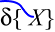
The sign 'd{ }' will again be used, and in much the same manner as it was in chapter I. For beta. purposes it will have a slight extension of usage. Used thus
the sign will represent a graph containing occurrences of the subgraph X, with a separate geodesic LI running from entirely outside the graph
to each of the relevant hooks in the subgraph X. If there are n such hooks in the whole graph thus represented, then there will be n separate geodesic LI's represented by the LI shown. If the sign is scribed in this manner:
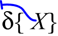
then it will indicate that all these LI's are connected by a "branching line" entirely outside the graph so represented.
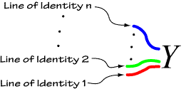
In the first case, then, the sign will represent a graph of form
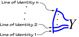
and in the second, one of form
By the alpha rules and beta Rbcl, then, we have
.gif) |
(9) |
Applying beta Ritr:
.gif) |
(10) |
Applying beta Rers, "breaking in even":
.gif) |
(11) |
Applying beta Rdit, "withdrawal of LI":
.gif) |
(12) |
And simple alpha iterations by Ritr:
.gif) |
(13) |
Now we prove another graph -- By the alpha rules:
.gif) |
(14) |
By beta Ritr, applied as often as necessary:
.gif) |
(15) |
Now another new graph -- First, again, by the alpha rules:
.gif) |
(16) |
And by beta Ritr as at step (15):
.gif) |
(17) |
Now apply beta Rnbc , "negative biclosure," as often as needed:
.gif) |
(18) |
We may now write the following graph as a specific case of graph (13) ;
.gif) |
(19) |
From the graph of (19) we may deiterate the graphs of (15) and (18) by Rdit
.gif) |
(20) |
But now with several applications of Rbcl, (20) becomes:
.gif) |
(21) |
An examination of the definition of the function g¢ will show us that when B is a member of the schema
|
|
(22) |
where a is free in A (and B is therefore a theorem of Fr), the graph of (21) will do very nicely as g¢ (B). This means that when B is a member of the theorem schema (22), g¢ (B) is a theorem of beta. But (22) is the case of the more general schema (2) when n = 1.
As we mentioned earlier, the extension of the procedure to any finite n offers no problem at all. The entire above proof may be executed showing any number of "parallel" LI's explicitly attached to X instead of the one that we actually showed. If we had shown two such LI's, for example, step (21) would be (with an extra biclosure )
.gif) |
(23) |
This, of course, would be g¢ of the schema
|
|
(24) |
The cases we have been discussing have been cases involving non-vacuous quantifiers. To show that g¢ of the schema of (2) is a theorem schema of beta when some of the quantifiers shown are vacuous would be quite simple, but irrelevant to the purpose of the lemma we are proving. We have indicated sufficiently, I think, that when D is a member of the theorem schema (2) of Fw, and all the quantifiers shown are non-vacuous, then g¢ (D) is a theorem of beta. We had already shown that if B is a member of the theorem schema (3) of Fw, then g¢ (B) is a beta theorem. By lemma 2.12, we know that R104, an analog in beta of the rule of detachment *104, exists as a derived rule of inference in beta. But by the remarks we made before we stated the present lemma, this means that if A is the closure of a tautologous wff of Fw, then g¢ (A) is a theorem of beta. And this is what we wanted to show.
The last lemma shows that the "axioms of quantification" admitted to Fw by Quine's *100 map into the set of theorems of beta by the one-one function g¢ , The next lemma will show that the same is true of the axioms of quantification admitted by *101.
| LEMMA 2.14 |
Whenever D is the closure of thr Fw
wff
then g¢ (D) is a theorem of beta. |
PROOF: We shall first prove this lemma for the
case where D is precisely the formula
![]() (a)(A
É
B)
É
. (a)A
É
(a)B
(a)(A
É
B)
É
. (a)A
É
(a)B![]() , Then we
shall show how it holds also in the cases where there are free variables in this
latter formula. For the case when there are no variables free in the
distribution formula: By the purely alpha clauses of the rules of
transformation:
, Then we
shall show how it holds also in the cases where there are free variables in this
latter formula. For the case when there are no variables free in the
distribution formula: By the purely alpha clauses of the rules of
transformation:
.gif) |
(1) |
Applying beta Rbcl:
.gif) |
(2) |
Applying beta Rers, " erasure in even":
.gif) |
(3) |
Applying beta Rdit, "withdrawal of LI":
.gif) |
(4) |
Extending branchings by Ritr, and applying Rbcl several times:
.gif) |
(5) |
The graph at (5) is g¢ (D) when D is the "distribution of universal quantifier over implication" formula, with no free variables. Actually, however, (5) as it stands is, strictly speaking, g¢ (D) only for the case in which the subformulas A and B of D contain only one occurrence each of the distributed variable a. It would be well for us to indicate that g¢ (D) will be a theorem of beta regardless of the numbers of occurrences of the distributed variable in A and B. We shall indicate how the proof may be so extended by assuming that A contains, say, three occurrences of the distributed variable, and B two. Then in place of (1) above, we shall scribe, by the alpha rules alone:
.gif) |
(6) |
Applying beta Rbcl as before:
.gif) |
(7) |
Now -- the characteristic step for these situations -- by beta Ritr:
.gif) |
(8) |
Note what we have done in step (8). We have iterated segments of LI into the annular space between the two cuts of the biclosure by clause 4 of beta Ritr. We may now easily by beta Rers and Rdit move to:
.gif) |
(9) |
By applying Rbcl as in step (5) this last graph becomes g¢ (D), where D is as hypothesized, with three occurrences of the distributed variable in A and two in B. It should be evident that this procedure may be extended to cover any possible combination of numbers of occurrences of the distributed variable in A and B.
The above proofs were, as we said earlier, proofs for the case where the distribution formula contains no free variables, is its own closure. We shall offer one example of a case where the distribution formula contains a free variable; let D be the cwff
|
|
(10) |
where b and only b is free in the distribution formula (with occurrences, say, in both A and B). The proof will be identical to the first we presented, except that we shall start out with a different first step. From our previous work (with lemma 2.13) it should be clear that the following is a beta theorem:
.gif) |
(11) |
It should be clear that each step of the first proof may be carried out without difficulty, beginning with (10), to come to the following result
.gif) |
(12) |
This last graph is
g¢ of (10) above, assuming
that there is one occurrence of a in each of A and B. For
cases involving different numbers of occurrences of a in A and B,
see steps (6) to (9) above and the remarks therewith. Note that
the operations of our proof do not disturb the LI's representing the occurrences
of b at all. It is clear that the procedure may be extended to any number
of free variables in the distribution formula, and we may consider the lemma
proven.![]()
We now move to a lemma which shows that the "axioms of quantification" admitted to Fw by *102 map into the set of beta theorems by g¢ .
| LEMMA 2.15 |
Where D is the closure of the Fw wff
|
PROOF: We present the proof only for the case
where there are no variables free in
![]() A
É
(a)A
A
É
(a)A![]() ; the
extension to cases where there are variables free presents no problem and is
quite similar to the analogous extension in the last lemma. Our explicit proof,
then, is for the case where D is the formula
; the
extension to cases where there are variables free presents no problem and is
quite similar to the analogous extension in the last lemma. Our explicit proof,
then, is for the case where D is the formula
![]() A
É
(a)A
A
É
(a)A![]() . The proof
involves one step; by the alpha rues alone,
. The proof
involves one step; by the alpha rues alone,
is a theorem of beta; this graph is
g¢ of
![]() A
É
(a)A
A
É
(a)A![]() . when a
is not free in A that is when the quantifier
. when a
is not free in A that is when the quantifier
![]() (a)
(a)![]() is vacuous. The double dead-end LI represents the vacuous quantifier according
to
g¢ .
is vacuous. The double dead-end LI represents the vacuous quantifier according
to
g¢ .
We now move to Quine's *103:
| LEMMA 2.16 |
When D is the closure of the Fw
wff |
PROOF: Once again, we shall show the proof only
for the case where the only free variable in
![]() (a)A
É
A¢
(a)A
É
A¢
![]() is b, that is,
where
is b, that is,
where ![]() (a)A
(a)A![]() contains no variables free. The extension to cases where there are other free
variables will be as in the preceding lemmas. By the alpha rules alone we have:
contains no variables free. The extension to cases where there are other free
variables will be as in the preceding lemmas. By the alpha rules alone we have:
.gif) |
(1) |
With beta Ritr and Rbcl we have:
.gif) |
(2) |
Applying beta Rers, breaking in even:
.gif) |
(3) |
Then, by beta Rdit, withdrawal of LI:
.gif) |
(4) |
And finally, Rbcl:
.gif) |
(5) |
The graph of (5) is
g¢(D) where
D is the cwff ![]() (b)((a)A
É
A¢
)
(b)((a)A
É
A¢
)![]()
The proof as sketched above is, of course, explicitly
for the case when A contains only one occurrence of a free. The
extension to cases where A contains more than one occurrence of a is
similar to that of steps (6) to (9) of lemma 2.14.![]()
We now have shown that all the axioms of quantification of Fw map into the set of beta theorems by the function g¢. We shall now show that the same is true for the "axioms of identity" as well.
| LEMMA 2.17 | When B is one of the Fw cwffs | ||||
|
|||||
| then g¢(B) is a theorem of beta. |
PROOF: The lemma will be proven by showing that the following proofs hold in beta:
By the alpha rules, we have
.gif) |
(1) |
Then, by Ritr:
.gif) |
(2) |
And applying Rbcl twice:
.gif) |
(3) |
The graph of (3) is
g¢(B) when B
is ![]() (a)(a = a)
(a)(a = a)![]() .
.
We shall state the proof for the second schema of this lemma only for the
case in which B itself is the formula
![]() (b)(a)(a =
b
(b)(a)(a =
b
.gif) |
(4) |
Applying Rbcl twice, we have:
.gif) |
(5) |
Applying beta Ritr and, again, beta Rbcl:
.gif) |
(6) |
The graph of (6), strictly speaking, is g¢(B) when B is the schema of substitutivity of identity with only one occurrence of a free in Aa and no variables free in B. We shall state simply that it is quite easy to extend the proof to any case of the substitutivity of identity. As an example, note a specific instance of this axiom schema:
![]() (y)(x)(x
= y
(y)(x)(x
= y
The graph corresponding to this formula is
which is easily provable in beta.![]()
We have now established that when A is either one of the axioms of quantification or the axioms of identity of Fw, then g¢(A) is a theorem of beta. But before we make use of the preceding lemmas in the proof of the central metatheorem of this section, let us examine briefly another issue which shall be of some importance in that proof.
Apart from the question of whether or not a given beta graph is a theorem of beta -- which is the question of whether or not there is a proof in beta for that graph -- we may raise the question of whether or not a given beta graph is valid. Although it is possible to speak of validity in a "purely syntactical" sense, it is undeniable that the notion -- even that of syntactical validity -- is intimately related to the interpretation of the system in question.
From what has gone before, we should have a good idea -- even without the formal statement of semantical rules -- of what the principal interpretation of beta will be. Beta graphs may be interpreted as statements, statements which are either true or false depending on "certain circumstances."
Speaking rather loosely, we might say that a given beta graph is valid iff it is true "regardless of what the circumstances are." It is incumbent upon us to be rather more specific however, in setting down just what it means to say, "The beta graph X is valid."
The first step in this direction will be to provide -- in definite terms -- a "sound interpretation" of the logic beta. According to Church,
we call an interpretation of a logistic system sound if, under it, all the axioms either denote truth or have always the value truth, and if further the same thing holds of the conclusion of any immediate inference if it holds of the premise.(n1)
The system Fr which we set down earlier in this chapter is a complete first-order calculus with identity; there are, of course, sound interpretations of Fr, Might it not be possible to provide our interpretation of beta through Fr, and thus avoid the statement of very complex semantical rules for beta? Indeed it is possible, and the means to do so are already at hand:
For a given sound interpretation of the system Fr, let the interpretation of the beta graph X be precisely the same as that of the Fr cwff f¢(X).
Such an interpretation of beta is unquestionably sound, for our metatheorem
*2.11 asserts that if a graph X is a theorem of beta, then
![]() r f¢(X).
This metatheorem guarantees that the conditions for soundness of an
interpretation are met by our suggestion for an interpretation of the beta
system., provided Fr has a sound
interpretation, which it has.
r f¢(X).
This metatheorem guarantees that the conditions for soundness of an
interpretation are met by our suggestion for an interpretation of the beta
system., provided Fr has a sound
interpretation, which it has.
Under this interpretation of beta, we may characterize validity in beta in this manner:
A beta graph X is valid iff the Fw cwff f¢(X) is valid.
We may then say, in effect, that validity is "preserved" through the function f¢. In the light of this, we may state quickly the following lemma:
| LEMMA 2.18 | Every theorem of beta is valid. |
PROOF: By our above remarks on validity in beta.![]()
Now we may move to the statement of the principal thesis of this section.
| *2.19 | The cwff A is a theorem of Fw iff g¢(A) is a beta theorem. |
"2.19 The cwff A is a theorem of Fw iff g¢(A) is a beta theorem.
PROOF: The "only if" part of this metatheorem follows immediately from lemma 2.12 -- which asserts the existence of detachment, or Quine' s *104., as a derived rule in beta --lemmas 2.13, 2.11, 2.15, and 2.16 -- which assert that the axioms of quantification admitted to Fw by Quine's *100, *102, and *103 respectively map into the set of beta theorems by g¢ -- and lemma 2.17, which asserts that the axioms of identity of Fw map by g¢ into the theorem set of beta. All the above means that if there is a proof for a cwff A in Fw, then there is a proof for g¢(A) in beta, and the "only if" part of the metatheorem holds.
Now, with the "only if" part holding, it is safe to say that we could, if we
wished, assign a sound interpretation to Fw by means of beta,
(through g¢) just as we
assigned an interpretation to beta through g¢.
We may say of the function g¢
-1, just as we did of f¢
-1, that "validity is preserved through it." If g¢(A)
is valid, then, so too will be the cwff A. If the "if'" part of this
metatheorem does not hold, then there is some cwff A of Fw
which is not a theorem of Fw while the graph g¢(A)
is a beta theorem. But Fw is a complete system, which is to
say that in it, every valid cwff is a theorem. So if A is not a theorem
of Fw, then A is not valid. By modus tollens,
then, g¢(A) must
be invalid. But this is impossible, since our supposition was that g¢(A)
is a beta theorem, and by lemma 2.18, every beta theorem is valid. Thus,
if A is not a theorem of Fw, then g¢(A)
cannot be a theorem of beta, and the metatheorem holds in both directions.![]()
2.34 The Completeness of Beta
As we stated in the rather trivial lemma 2.18, every beta theorem is valid. But more interesting than this is the question of whether or not every valid beta graph is a theorem; equivalently, this is the question of whether or not beta is complete. We shall now answer that question in the affirmative:
| *2.20 | Beta is complete. |
PROOF: As we have remarked, beta is complete iff every valid beta graph is a theorem of beta; this we shall now prove. To avoid interrupting the general development with a long graphical proof, we shall, for the moment, assume the following, for which demonstrations shall subsequently be provided:
| 1. |
|
||||
| 2. |
There is a (many-one) function k taking the set of beta
graphs as its domain and
|
||||
|
Suppose that a beta graph X is valid (recall from our earlier remarks that a beta graph X is valid iff f¢(X) is a valid cwff). Then, by 2-b above, k(X) is also valid. But
k(X)
Î
![]() b
b
that is, there is a cwff A of Fw such that k(X) is the
same graph as g¢(A); g¢(A), being precisely
k(X), is valid. But then, as we remarked in
the proof of *2.19, A itself must be valid, and so by the completeness of
Fw, A
must be a theorem of Fw. By *2.19, then, g¢(A) -- and so too
k(X), which is g¢(A) -- must be a theorem of beta. But if
k(X) is a theorem of beta, then -- by 2-a
above -- so too must X be a theorem of beta. Therefore, if a beta graph
X is valid, it must be a theorem of beta, and beta is complete. The
completion of this proof awaits the demonstration of 1 and 2 above, which will
follow an immediate corollary.![]()
| COROLLARY 2.21 | If the cwff f¢(X) is a theorem of Fr, then the graph X is a theorem of beta. |
PROOF: Immediate: Every theorem of Fr is a valid cwff, so if f¢(X) is a
theorem, f¢(X) is valid. But then the beta graph
X is also valid, and by *2.20 is a beta theorem.![]()
This last corollary is the long awaited converse of *2.11, and in conjunction with *2.11, it establishes that "A beta graph X is a theorem of beta iff f¢(X) is a theorem of Fr."
We now move to assumptions 1 and 2 in the proof of *2.20. We shall first work
with the first of these assumptions, that is, that the set
![]() b
is recursively characterizable. We shall show that it is so characterizable by
presenting a set of rules which characterizes it; these rules will be exactly
parallel respectively to the rules characterizing the set of cwffs of the system
Fw.
b
is recursively characterizable. We shall show that it is so characterizable by
presenting a set of rules which characterizes it; these rules will be exactly
parallel respectively to the rules characterizing the set of cwffs of the system
Fw.
The major problem here is that the cwffs of Fw are defined through the wffs in general, and there are wffs of Fw which are not closed; as we have indicated, however, there is no beta graph which is not a "closed formula."
We shall require a device in our characterization, then, to parallel the free variable of Fw. This device we shall call the "free LI terminal," or "flt."
If a spot has attached to any of its hooks an LI which crosses no cuts and comes to a dead end without branchings or connections, that dead end will be called an flt. If either of the two LI ends extending from the graph
comes to a dead end without cut-crossing, branching, or connections, it too will be called an flt. Only these termini will be called flts.
Note carefully that the flt is by no means to be considered to be related to
the free variable of Fw by g¢
-- it is merely an expedient we employ to help us define the set
![]() b.
We shall now define a set Q of beta graphs, of which
b.
We shall now define a set Q of beta graphs, of which
![]() b
is a subset, just as the cwffs of Fw are a subset of the wffs.
We shall in each case state a rule of formation of Fw, and
with it, the analogous rule for Q.
b
is a subset, just as the cwffs of Fw are a subset of the wffs.
We shall in each case state a rule of formation of Fw, and
with it, the analogous rule for Q.
| 2.34i | Fw rule: | 'Æ' (constant false proposition) is wf. | ||||||||||||
| Q rule: | The empty cut, '
|
|||||||||||||
| 2.34ii | Fw rule: |
|
||||||||||||
| Q rule: |
|
|||||||||||||
|
|
||||||||||||||
| 2.34iii | Fw rule: |
Where A is a predicate symbol of degree n, and a1,
a2, . . ., an are n individual
variables, |
||||||||||||
| Q rule: |
|
|||||||||||||
| 2.34iv | Fw rule: | Where j and y are both wf, Cjy is wf. | ||||||||||||
| Q rule: |
|
|||||||||||||
| 2.34v | Fw rule: |
Where A is wf and a is an individual variable,
|
||||||||||||
| Q rule: |
|
|||||||||||||
| 2.34vi | Fw rule: | (Understanding the meaning of "free variable") Where A is wf and contains no free variables, A is a closed wff, or cwff. | ||||||||||||
| Q rule: |
Where X is a member of Q, and X contains no flts ,
X is a member of
|
This completes the definition of the set
![]() b. The "proper ordering" referred to in
2.34v is meant to agree with the similar "ordering of connections" required in
the definition of the function g
b. The "proper ordering" referred to in
2.34v is meant to agree with the similar "ordering of connections" required in
the definition of the function g
The above recursive characterization takes care of assumption 1 in the proof
of *2.20. We shall now move on to the second of these assumptions. This
is that there is a function k with the set of beta graphs as its
domain and the set
![]() b,
as its range such that
b,
as its range such that
| (a) | X is a beta theorem iff k(X) is a beta theorem, and |
| (b) | X is a valid graph iff k(X) is a valid graph. |
Because of the large variety of sign-complexes possible in beta, the demonstration that k exists will be largely a matter of busy-work, which we now enter into.
First of all, let us specify that if X is a member of
![]() b,
then k(X) = X. For graphs which are already members
of
b,
then k(X) = X. For graphs which are already members
of
![]() b,
then, there is no problem. For them k is simply the identity
function, and trivially possesses the required properties.
b,
then, there is no problem. For them k is simply the identity
function, and trivially possesses the required properties.
For graphs which are not members of the range of g¢,
however, proving the existence of k is another problem. Our method
will be to show that with applications of the beta rules of inference alone, any
beta graph X as premise has as a consequence a member of
![]() b,
which we shall call k(X); and further, that k(X)
as premise, by applications of the beta rules alone, has as a consequence the
graph X. If this is the case, then obviously, X is a beta theorem
iff k(X) is a beta theorem; this is one of the required
properties of k.
b,
which we shall call k(X); and further, that k(X)
as premise, by applications of the beta rules alone, has as a consequence the
graph X. If this is the case, then obviously, X is a beta theorem
iff k(X) is a beta theorem; this is one of the required
properties of k.
We also wished k to be such that X is valid iff k(X) is valid. If the computation of k(X) from X consists solely in a deduction from X as premise by the beta rules of transformation, and if, with k(X) as premise X can be derived by the beta rules alone, then it is indeed the case that X is valid iff k(X) is valid. If R(Y, X) is one of the beta rules, then, as we have shown for each of these rules, if f
¢(X) is a theorem of Fr, then so too is f¢(Y). Suppose X to be valid; then f¢(X) must also be valid, by our definition of validity in beta. (since we have agreed that the interpretation of any beta graph is to be exactly the same as that of f¢ of that graph). By the completeness of Fr, then, f¢(X) is a theorem of Fr. Then if for some Y, R(Y, X) is true, then also f¢(Y) is a theorem of Fr. But then f¢(Y) is trivially valid, and so too then is Y. We conclude then that no consequence of a valid beta graph by the beta rules of inference can be invalid, and so as we have suggested k should be, X is valid iff k(X) is valid.We know, then, that if k(X) is computed by taking X as a premise and applying the beta rules of transfomation, and if with k(X) as a premise X may be deduced by the beta rules alone, then both of the properties required of our function k in the proof of *2.20 are there, that is, X is a beta theorem iff k(X) is, and X is valid iff k(X) is.
It is now a question of showing that any beta graph as premise may be
transformed into a member of
![]() b
by the beta rules alone, and that that member of
b
by the beta rules alone, and that that member of
![]() b
as premise may be transformed back into X by the beta rules of
transformation alone.
b
as premise may be transformed back into X by the beta rules of
transformation alone.
We now take an arbitrary beta graph X which is
not a member of
![]() b.
We may say this: if X is to be transformed into a member of
b.
We may say this: if X is to be transformed into a member of
![]() b,
then there must be transformations available which will enable us, first, to get
the LI network of X into a pattern characteristic of a member of
b,
then there must be transformations available which will enable us, first, to get
the LI network of X into a pattern characteristic of a member of
![]() b
, and secondly, to transform the cut-nest of X into a cut-nest
characteristic of a member of
b
, and secondly, to transform the cut-nest of X into a cut-nest
characteristic of a member of
![]() b.
b.
We first approach the problem of the LI network. We shall do this in steps
| Step 0: | If X is of form | ||||||||
|
|
|||||||||
| let it as it is; otherwise, transform it to | |||||||||
|
|
|||||||||
| Step 1: | The "cyclic graph" step. If there are any cyclic graphs in X, convert them to double-dead-end LI ' s by Ritr and Rdit thus: | ||||||||
|
|
|||||||||
| Step 2: | The "dead end" step. If a dead end occurs in a given area of the graph resulting from the previous steps, then for that area we have one of the following forms, where W is the entire graph in that area apart from the dead end in question (note that W could be as little as the "other end" of a double-dead-end LI, or even, in some cases, the null-graph), and -- in (2) below -- Z is the graph, whatever it might be, which is outside the area in question, and to which the dead end in question is connected. We thus have, for a given dead end in a given area, either | ||||||||
|
|||||||||
| These may be transformed by Rbcl respectively to | |||||||||
|
|||||||||
| Now, in some established order, carry out the applicable one of the transformations above for each individual dead end in the graph resulting from step 1. | |||||||||
| Step 3: | The "branching" step. If a branching occurs in a given area of the graph resulting from the previous steps, then for that area we have one of the following forms, where W is as in step 2, and X, Y, and Z all have the function of Z in step 2. | ||||||||
|
|||||||||
| By Rbcl, these may be transformed respectively to | |||||||||
|
|||||||||
| Now, in some established order, carry out the applicable one of the above transformations for every individual branching in the graph resulting from step 2. | |||||||||
| Step 4: | The "connecting LI" step. In the graph resulting from the previous steps, there may be places where two graphs in the same area, Y and Z, are connected by a LI which has its outermost portion in the same area in which Y and Z occur. This is case (7): | ||||||||
|
|
|||||||||
| By Rbcl, this may be transformed into (7¢): | |||||||||
|
|
|||||||||
| Now, in some established order, carry out the above transformation for every case in the graph resulting from the previous steps where two graphs are connected as in (7). | |||||||||
| Step 5: | The "in-pointing loop" step. In the graph resulting from the above steps, there may be cases where there are loops with "their ends pointed in" -- if step 4 had to be applied, there will indeed be such loops. For a given area into which such a loop points, using W as before, we have (8) | ||||||||
|
|
|||||||||
| By Rbcl, this may be transformed to (8¢): | |||||||||
|
|
|||||||||
| For every such in-pointing loop in the graph resulting from step 4, in some established order, carry out the above transformation. Note that if at (8) there were two such loops, the final result of the transformation would look like | |||||||||
|
|
|||||||||
| Step 6: | The "quantifier-indicating" step. In the graph as so far transformed, dead-ends, "in-pointing" loops (those of step 5). and branchings all occur, respectively in subgraphs of the forms, now to be shown, where the dead end, loop, or branching is the only sign in the annular space between the two cuts shown with the possible exception of geodesic LI's which pass from completely outside the outer to completely inside the inner of the cuts. The operations to this point have been arranged, then, so that the dead end, in-pointing loop, or branching is the only graph standing in that annular space. Each dead end, in-loop, or branching of the graph, then, occurs, respectively in a subgraph of form | ||||||||
|
|||||||||
| By Ritr these may be transformed into | |||||||||
|
|||||||||
| At this point a
striking similarity to something we saw in rule 5 of the characterization
of
|
|||||||||
| Step 7: | The "out-pointing loop" step. All loops remaining in the graph as it now stands are "out-pointing"; where such a loop occurs in a given area, we have (using W, Y, and Z as before ) (12): | ||||||||
|
|
|||||||||
| By Rbcl this is transformable to (12¢): | |||||||||
|
|
|||||||||
| Note that if 2 such loops stand in the same area as W, (12¢) will be | |||||||||
|
|
|||||||||
| Transform every loop remaining in the graph resulting from step 6 as above. |
I contend that we have now transformed -- using Rbcl, Ritr,
and Rdit alone -- the LI network of the original graph into an
LI network characteristic of a member of
![]() b.
Note that all branchings and dead ends in the transformed graph occur in
subgraphs of form (9'). (10'). or (11') above. This is precisely as is required
for the branchings and dead ends of a member of
b.
Note that all branchings and dead ends in the transformed graph occur in
subgraphs of form (9'). (10'). or (11') above. This is precisely as is required
for the branchings and dead ends of a member of
![]() b
by rules 5 and 6 characterizing
b
by rules 5 and 6 characterizing
![]() b.
Note too that all the loops in the graph we now have occur only in
subgraphs '
b.
Note too that all the loops in the graph we now have occur only in
subgraphs '![]() ', by step
7. This also is as required by the characterization of
', by step
7. This also is as required by the characterization of
![]() b.
Any LI which crosses a cut -- apart from those in the subgraphs '
b.
Any LI which crosses a cut -- apart from those in the subgraphs '![]() '
-- is geodesic, and moves inwards from one of the branching complexes '
'
-- is geodesic, and moves inwards from one of the branching complexes '![]() ',
'
',
'![]() ', or '
', or '![]() '
as they occur in the forms (9'). (10' ), and (11' ) to connect either to a hook
of a spot or to one end of the graph Thus I submit that we have transformed the
LI network of the original graph into an LI network characteristic of a member
of
'
as they occur in the forms (9'). (10' ), and (11' ) to connect either to a hook
of a spot or to one end of the graph Thus I submit that we have transformed the
LI network of the original graph into an LI network characteristic of a member
of
![]() b.
What follows is easy. The steps required to make the graph as it now stands a
member of
b.
What follows is easy. The steps required to make the graph as it now stands a
member of
![]() b
are almost the same as the steps by which any alpha graph may be transformed
into a member of
b
are almost the same as the steps by which any alpha graph may be transformed
into a member of
![]()
I shall go no further here than to offer the argument that just as any wff containing only the connectives 'K' and 'N' may be transformed into an equivalent wff containing only the connective 'C' and the constant false proposition '
Æ' merely by application of the law 'EpNNp' through substitutivity of equivalence and the equivalences 'ENNKpNNqNCpNq' and then 'ENpCpÆ', so too may any graph resulting from the application of our seven steps be converted, by Rbcl alone, to a member ofThus we will argue that the function k required for the proof
of the completeness of beta exists, and has the properties required of it. We
have shown explicitly that an arbitrary graph X may be converted by the
beta rules Rbcl, Ritr, and Rdit
alone into a member of
![]() b,
which we may call k(X). And since the above mentioned rules
are all that are required to do the job, with k(X) as a
premise, X may be derived, since the converse of each of the rules used
is itself a rule of beta; the proof of X from k(X)
is then just the "reverse" of that of k(X) from X.
We have thus shown that with an arbitrary beta graph X as premise,
k(X) such that k(X) is a member of
b,
which we may call k(X). And since the above mentioned rules
are all that are required to do the job, with k(X) as a
premise, X may be derived, since the converse of each of the rules used
is itself a rule of beta; the proof of X from k(X)
is then just the "reverse" of that of k(X) from X.
We have thus shown that with an arbitrary beta graph X as premise,
k(X) such that k(X) is a member of
![]() b
may be computed using the beta rules alone, and that if that k(X)
is taken as a premise, X may be derived by the beta rules alone.
Therefore, as required in the metatheorem on completeness, there is a k
such that for any X, k(X)
b
may be computed using the beta rules alone, and that if that k(X)
is taken as a premise, X may be derived by the beta rules alone.
Therefore, as required in the metatheorem on completeness, there is a k
such that for any X, k(X)
2.35 The Intertranslatability of Beta and First Order Calculi with Identity
Recalling Martin Davis's definition of translatability, which we employed in chapter I, we may state the following metatheorem:
| *2.22 | Beta is translatable into any complete classical first-order calculus with identity, and any such calculus is translatable into beta. |
PROOF: Immediate. the functions f
¢ and g¢ are both one-one functions, as required in the definition of translatability, and we have proven that: X is a beta theorem iff f¢(X) is a theorem of Fr, which means, by the definition, that beta is translatable into Fr, We have also proven that a cwff A is a theorem of Fw iff g¢(A) is a theorem of beta, which means that Fw is translatable into beta. But Fw and Fr are translatable into each other, and into any full classical first-order calculus with identity, and any such calculus is translatable into either Fw or Fr, By the transitivity of translatability, then, the metatheorem holds.| COROLLARY 2.23 | The decision problem for beta is recursively unsolvable. |
PROOF: By Martin Davis's theorem 8.1.3,(n1)
*2.22, and the recursive unsolvability of the decision problem for full
first-order calculi.![]()
This chapter has been quite an effort--for reader as much as for author, I am sure -- but I believe that it has been worth it. It has established that the unlikely looking system beta is, in effect, a full first-order calculus with identity. And it has introduced us to and shown us the power of a novel concept in symbolic logic -- that of implicit quantification as exemplified in the beta line of identity.