OUR detailed study of the existential graphs as formal systems begins with alpha. This chapter will be devoted to a comparison of alpha with the classical propositional calculus (which we shall ordinarily abbreviate by "CPC" or simply "PC"). Alpha, as we shall see, is a logic; the rules of transformation for alpha presented in the Introduction are the rules of inference of that logic. As a logic, alpha has theorems, theorems provable through those rules of transformation; we shall see how those theorems are related to those of CPC.
"Project alphas" then, is an examination of relationships existing between alpha and the ordinary CPC, Obviously, since the notation of alpha is very different from that of garden variety logics, the first thing we must do is to find a means of "translating" alpha graphs into wffs of ordinary PC's and vice-versa.
We describe a function, or set of instructions, which will enable us to translate any alpha graph into a unique formula of the PC; this function we call "f." In describing this function, we first show how to write "names" of alpha graphs, and then we designate a set of these names as "standard" names; the designation is such that each alpha graph has one and only one standard name. we then show how to transform standard names into unique CPC wffs. If X is any alpha graph. then the CPC wff formed by applying these instructions to X will be called f(Y).
At this point we will note that in our work with alpha we will set out and use two different formulations of the CPC rather than just one. The first of these systems is one which has conjunction and negation as primitive operators; this formulation is called Pr (the "r" is for Rosser). The other system uses implication as a primitive operator and has a primitive constant false proposition; this formulation is called Pw (the "w" is for Wajsberg). Pr and Pw are both complete CPC's, and as such are "equivalent." The reason we use two systems rather than just one is one of convenience. Pr is a convenient system into which to translate alpha graphs in one-one fashion; for a given alpha graph X the formula f(X) will be a wff of Pr. But Pw is a convenient system from which to translate wffs into alpha graphs in one-one fashion, as we shall see.
We have mentioned that we shall describe a function f which "translates" alpha graphs into wffs of the system Pr. We shall also describe a one-one function, or set of instructions, which will enable us to translate any wff of the system Pw into a unique alpha graph; this function we shall call "g." Where A is any wff of Pw, the unique graph formed by applying this set of instructions to A will be called g(A).
We shall provide a precise definition of what it means to be a logic, and we shall show how alpha "fits" this definition; that is, we shall show that alpha is a logic. In the process of doing this, we shall sat down precise formulations of the alpha rules of transformation which -- as we have mentioned -- are the rules of inference of the logic alpha.
Certain of the alpha graphs will be theorems of the logic alpha. Through a series of lemmas we shall establish that:
The graph X is a theorem of alpha iff the wff f(X) is a CPC theorem.
We shall also establish that:
The wff A is a CPC theorem iff the graph g(A) is a theorem of alpha.
We shall thus have established that the set of theorems of alpha maps one-one into the set of theorems of the CPC, and vice-versa. This means that given the natures of the functions f and g, alpha itself may be considered a complete classical CPC.
1.1 The Set of Alpha Graphs
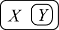
'We may first note that involved In the makeup of alpha as we have examined it is a set of objects, objects which are simply certain signs and combinations of signs that may be scribed, say, upon a sheet of paper or a blackboard. Consider a denumerably infinite set, Ma, of such signs, which we will denote individually by the letter 'b' followed by a sequence of primes, which sequence may be null. The members of the set Ma, then, are b, b¢, b¢¢, . . .. It is understood, of course, that the correlation of the members of Ma to the signs 'b', 'b¢ ', etc. is strictly one-one. No member of Ma is analysable into "smaller" signs, so we may call Ma the set of "minimal" or "atomic" graphs of alpha. The first member of this set, b, has a special status; it is the "null-graph" or "blank." Recall that the blank SA is to be considered a graph. The other members of Ma, b¢, b¢¢, . . ., may be considered "graph-variables," with a function not unlike that of the propositional variables of the ordinary CPC. In the present treatment, we shall generally employ upper-case letters 'X', 'Y ', etc. as variables of the metalanguage ranging not only over the members of Ma, but over all objects which may come to be called graphs as well.
Consider now another sign of the metalanguage. Let S(X) be "the result of enclosing the graph X by the ordinary alpha cut," which as we learned in the Introduction is a "self-returning linear separation" scribed upon the surface upon which we are working. Please note that if two "self returning linear separations" intersect each other, neither qualifies as a "cut," The cut itself is not a graph, but it plus the graph it encloses is a graph; that is, the scribing of a cut around a graph is a "graph-forming operation." Note that in practice a cut cannot be scribed without forming a graph, for it will always enclose at least b, the null-graph.
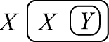
If a graph X Is enclosed by a cut, and another graph Y lies outside that same out, we shall say that X and Y are "separated"; otherwise they are "unseparated." This brings us to another sign of the metalanguage. Where X1, . . ., Xn are n alpha graphs, each of which is either of the form S(Y) or is a member (other than b) of the set Ma, then J(X1, . . ., Xn) is "the result of scribing the n graphs X1, . . ., Xn unseparated on SA." The operation of scribing graphs unseparated on SA is then also a "graph-forming" operation.
We may summarize the above by listing the following rules; these rules may be considered the rules characterizing the set of alpha graphs:
| 1.1i | Each member of the set Ma is an alpha graph. | |
| 1.1ii | Where X is an alpha graph, S(X) is an alpha graph. | |
| 1.1iii | Where X1, . . ., Xn are n alpha graphs other than b admitted by rules 1.1i or 1.1ii, thenJ(X1, . . ., Xn) is an alpha graph. |
From what has gone before„ we should already have a good idea of how to go about naming an alpha graph, as we have actually been using names of alpha graphs in our development. But we shall list some explicit rules similar to the above which will tell us formally how graphs are named.
| 1.1iv | 'b' names the null-graph; 'b', followed by one prime or more, names a member of Ma; 'b' followed by n primes names the same graph as 'b' followed by m primes iff n = m. | |
| 1.1v | The sequence of signs consisting of 'S(' followed by the name of the graph X followed by ')' names a graph; specifically, it names the graph formed by enclosing X by an alpha cut. | |
| 1.1vi | Where the graphs X1, . . ., Xn are n, n ³ 2, graphs admitted by rules 1.1i or 1.1ii, and none of them is the null-graph then the sequence of signs consisting of 'J(' followed by the n names of the X1, . . ., Xn followed by '}' names a graph; specifically, it names the graph formed by scribing the X1, . . ., Xn unseparated on SA. |
Now note that since the set of alpha graphs is characterizable by the rules 1.1i-1.1iii it is a recursive set. Since it is recursive, it may be ordered (every recursive set is recursively enumerable in increasing order without repetitions) in such a manner that alpha graphs X and Y are associated with the same natural number iff X and Y are identical, that is, are able to be "generated" by exactly the same applications of rules 1.1i-1.1iii. We could, if we wished, describe means for such an ordering. Such a description would, however, be long, tedious, and irrelevant. The important thing is to know that the set may be so ordered; the exact "how" of the ordering does not make too much difference. Let us then select some ordering of the alpha graphs such that each alpha graph is associated with a unique natural number, and vice-versa. If, then, the names of the a alpha graphs X1, . . ., Xn are written in a sequence, we shall see that that sequence is "properly ordered" iff it is ordered according to our selected unique ordering of alpha graphs. Of course, for any n such graphs there is one and only me "proper ordering."
We shall now define what we shall call the "standard name" of an alpha graph:
| 1.1vii | The names of graphs admitted by 1.1iv are standard names. | |
| 1.1viii | The sequence of signs consisting of 'S(' followed by the standard name of the graph X followed by ')' is a standard. name. | |
| 1.1ix | Where X1, . . ., Xn are n, n ³ 2, alpha graphs admitted by rules 1.1i or 1.1ii, and none of them is the null-graph, then the sequence of signs consisting of 'J(' followed by the n standard names of the X1, . . ., Xn followed by ')' is a standard name, provided the sequence of n names between the 'J(' and the ')' is properly ordered. |
It should be evident that each alpha graph has one and only one standard name,
A question worth noting at. this point is that of the cardinality of the get of alpha graphs. Although we have asserted that this set is recursive, and so at most denumerably infinite, the graphical nature of the system may well conjure up ghosts of the power of the continuum to haunt us. Lot us simply remark here that our study involves only graphs containing a finite number of signs -- an assumption well-grounded in the study, say, of the ordinary logical systems, which deal only in finitely long words or sentences. Since this is the case, It is impossible that the number of alpha graphs be larger than a denumerable infinity. We may seem in this to be somewhat less liberal than Peirce himself, who seems at one point to indicate that graphs containing infinitely many signs are permitted (4.494). We must comment, however, that there are marked differences between the presentation of a system permitting wffs of finite length only, and that of one permitting infinitely long wffs. What Peirce says in 4.494 is certainly a rather casual remark, the full implications of which did not occur to Peirce when he made it -- and hardly could have, since the study of systems containing infinitely long sentences is of rather recent vintage. Indeed, so far as I have been able to determine, ho does not mention the matter again in the writings on the graphs included in the Collected Papers. We shall thus stick by our assumption that an alpha graph may be of finite length only.
1.2 The Alpha Graphs and the WFFS of the Classical Propositional Calculus
We shall begin by setting out two systems of complete CPC; these systems will
be called, respectively, Pr and Pw. The
respective sets of wffs for these systems will be called (Pr)
and (Pw). We shall employ the upper-case letters of the Roman
alphabet (or lower-case Greek letters) as variables ranging over the CPC wffs. "![]() r
A" shall be read, "A is a theorem of Pr," and "
r
A" shall be read, "A is a theorem of Pr," and "![]() w
j" shall be read, "j is a theorem of Pw." The
"primitive signs" of Pr include a denumerable infinity of
signs, p0, p1 p2, . . .,
called "propositional variables," left and right parentheses, '(' and ')' and
the sign '~',
called "the negation sign" The rules of formation for Pr are:(n1)
w
j" shall be read, "j is a theorem of Pw." The
"primitive signs" of Pr include a denumerable infinity of
signs, p0, p1 p2, . . .,
called "propositional variables," left and right parentheses, '(' and ')' and
the sign '~',
called "the negation sign" The rules of formation for Pr are:(n1)
| 1.2i | pi is wf, i ³ 0. | |
| 1.2ii |
|
|
| 1.2iii |
|
Definitions will be as usual in the CPC, with a definition considered as providing a notational abbreviation for a formula in primitive notation; where there is no danger of confusion, we shall employ the staple letters 'p', 'q', 'r', 's', . . . as propositional variables in place of the primitive p1, p2, p3, . . .. As with all definitions, this is to be understood to be a space and time saving abbreviation. The variable p0 will have a special use in this system, in the following definition:
1 =df ~(p0~(p0)).
As rules of inference, Pr shall have substitution for variables and detachment; the axioms shall be Rosser's set:
| p É .p.p | ||
| p.q. É p | ||
| p É q. É .~(qr) É ~(rp) |
Note that we have presented the axioms in definitionally abbreviated form rather than in primitive notation.
The primitive signs of Pw are, propositional variables, a sign 'Æ', called the "constant false proposition," and a sign 'C', called the "sign of implication." The rules of formation are:
| 1.2iv | pi is wf, i ³ 0. | |
| 1.2v | Æ is wf. | |
| 1.2vi |
|
Again, standard definitional abbreviations will be used, including the use of p, q, . . . as notational shorthand for p1, p2, p3, . . .: the rules of inference are substitution and detachment, and the axioms are:
| CCpqCCqrCpr | ||
| CpCqp | ||
| CCCpqpp | ||
| CÆp |
we are now prepared to note down a means of moving from the alpha graphs to the wffs of the CPC and vice-versa, we define a recursive word function f:
| D1: | The function f takes the set of alpha graphs an its domain, and finds its range in the set (Pr). Given any alpha graph X, write the standard name of X. Wherever in that standard name the "subname" J(Y1, . . ., Yn) occurs, for all such "subnames" involving 'J', delete the 'J(' and the ')'s leaving Just the sequence Y1, . . ., Yn. Wherever 'S' occurs, replace it with the sign '~'. Wherever the simple 'b' occurs, replace it by '1', that is, by ~(p0~(p0)). Wherever 'b' occurs followed by i primes, i ³ 1, replace that occurrence of 'b' and the primes following it by pi, This completes the instruction for f; the result of the application of this instruction to an alpha graph X will be called f(X), end is a wff of Pr. |
This last definition tells us how to transform an alpha graph into a wff of the CPC. As we remarked earlier, there to one and only one "standard name" for each alpha graph. It is quite clear that given any standard name, the latter part of the instructions in Dl will yield one and only one wff of Pr, The function f as defined above, then, is a one-one function; f(X) will be the same formula as f(Y) iff X is the some graph as Y. The intuitively acceptable interpretations of the signs of the alpha graphs are preserved in the translation made possible by the function f; unseparated occurrence of graphs in an area is correlated by f to PC conjunction, and enclosure by a out is correlated to inclusion in the scope of a negation sign; the minimal graphs of alpha are correlated to the atomic formulas of Pr.
We now mow on to the definition of the function which will enable us to
translate wffs of the CPC into alpha graphs, First of all, we shall consider a
subset of the set of alpha graphs, which we shall call
![]() a.
Membership in
a.
Membership in ![]() a
is defined as follows:
a
is defined as follows:
| 1.2vii | All members of the
set
Ma are members of
|
|
| 1.2viii | S(b)
is a member of |
|
| 1.2ix | If X and
Y are both members of
|
Let us introduce the following definitton:
| D2: | G(XY) =df S(J(XS(Y))) |
We might now restate the last rule thus: If X and Y both
are members of ![]() a
, then G(XY) is a member of
a
, then G(XY) is a member of
![]() a.
a.
We may now move directly to a statement of the function g:
| D3: |
The function
g takes (Pw) as its domain, and
|
It is clear that the function g is one-one and onto
![]() a.
a.
1.3 Alpha as a Logic
Before entering into a detailed study of alpha as a logic, it will be well to may a few words about logics in general. The definitions we employ are in general adopted from Martin Davis; we retain, however, our numbering, First of all, let us say what we mean by "logic."(n1)
| D4: | By a logic
|
It should be clear that a "recursive word predicate" is to a number-theoretic predicate as a recursive word function is to a (partial recursive) number-theoretic function.
| D5: | When R(Y,
X1, . . . , Xn) is a rule of inference
of |
|||||
| D6: | A finite sequence
of words X1, X2, . . ., Xn
is called a proof in a logic
|
|||||
|
||||||
| D7: | We say that W
is a theorem of |
|||||
|
||||||
| if there is a
proof in |
1.31 "Theorem Generation" in Alpha
It will be our desire to show to quickly as possible that alpha is a logic. But before we state a metatheorem to this effect, lot us examine alpha in the light of the requirements of Davis's definition. The first such requirement is for a recursive set of axioms; the usual criterion for determining what -- in a given system -- is an axiom is the word of the author of the system. Peirce was not so kind as to say explicitly, "Such-and-such a graph is an axiom of alpha," so we must look closely at the matter. An axiom is a theorem or "assertable word" of the system which need not be derived or proven within the system. Examining Peirce's presentation of alpha, we find one end only one graph which qualifies as such in what may be called the "unspecialized version" of alpha (that is, alpha with no "extralogical" premises). That graph is the blank sheet of assertion itself. We will recall that Peirce explicitly called SA a graph, and that we have notation in our metalanguage to speak about it. Any blank area on SA (and this includes the completely blank SA itself) is the null-graph, or b. Since SA is a presupposition of any graph whatsoever, we shall declare that the axiom set of alpha contains one and only one member, b.
It may seem curious to employ a null "something-or-other" as an axiom, since we very commonly think of the null-set as correlated in some way with the truth-value "false"; but let us recall that the "constant false proposition" employed in many systems of PC is often explicated as the proposition which says that "everything is true." This explication is exemplified in systems which have quantifiers ranging over propositional variables; in these systems the proposition '~(p)p' is a theorem. In the sense of "null" which is contrasted to the above sense of "universal," then, it is quite reasonable to take the "null-graph" as assertable.
The other requirement of Davis's definition of a logic In that it contain a finite set of recursive word predicates, the rules of inference of the system. It is clear that the rules of transformation for alpha qualify as such recursive word predicates. Employing 'R' with a subscript as notation for these predicates, we may list them as follows:
| Rins(Y, X): | Which is true iff Y is identical to X except for containing in a position enclosed by an odd number of cuts a graph Z which X does not contain at the corresponding position. | |
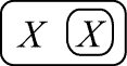
| Ritr(Y, X): | Which is true iff X is identical to X except for containing one more occurrence of a subgraph Z than does X (with X having at least one occurrence of Z); the extra occurrence of Z in Y is to be located in an area enclosed by at least all the cuts which enclose another occurrence of Z in Y, which last mentioned occurrence corresponds to an occurrence of Z in X. | |
| Rbcl(Y, X): | Which is true iff Y is identical to X except for containing a graph S(S(Z)) where X contains simply Z. |
The above predicates may be called the "positive rules of inference in alpha." In addition, we have the following "negative" rules:
| Rers(Y, X): | Which is true iff Rins(S(X), S(Y)) is true. | |
| Rdit(Y, X): | Which is true iff Ritr(X, Y) is true. | |
| Rnbc(Y, X): | Which is true iff Rbcl(X, Y) is true. |
The above six predicates are easily recognised respectively as Peirce's rules of insertion in odd, iteration, biclosure, erasure in even, deiteration, and negative biclosure. we may now state the following metatheorem:
| *1.01 | Alpha is a logic. |
PROOF: By D4 and the above exposition of
axiom and rules of inference in alpha.
![]()
The axiom of alpha, then, pines us a starting paint from which. we may, by the stated rules of inference of alpha, generate the theorems of alpha. We now enter into an investigation of that set of theorems of alpha.
1.32 The Logic Alpha in the System Pr
In D1 we defined a function f which maps the set of alpha graphs into the set of wffs of Pr. Our project is now to show that whenever a given alpha graph X is a theorem of alpha, the corresponding wff, f(X), is a theorem of Pr, and then to show the converse, that whenever f(X) is a theorem of Pr, X is a theorem of alpha.
| LEMMA 1.02 | f (b) is a theorem of Pr. |
PR00F: By D1, f (b)
is '1', which is '~(p0.•
~p0)',
which is immediately recognized as a theorem of Pr.![]()
The above lemma establishes that the axiom of alpha is correlated by f to a theorem of Pr. We now turn to the rules of inference in alpha, proving in the process two lemmas that are of some independent interest in the study of the CPC itself. We shall say that a given occurrence of wf subformula, B, of Pr is in "antecedental position," or "A-pos," in a Pr wff Q, and we shall write QA(B) for the whole formula iff the occurrence of the subformula B is within the scope of an odd number of negation signs in Q at the one occurrence of B in Q which is in question. We shall say that that occurrence of B is in "consequential posit ion," or "C-pos," and shall write QC(B) for the whole formula otherwise, that is, when B is in the scope of an even number of, or of no negation signs in Q.
| LEMMA 1.03 |
Where |
| LEMMA 1.04 |
Where
|
PROOF: These two lemmas shall be proven together. It is understood, of course, that in each lemma the D is to be considered as replacing the B.
We know that it is possible to reduce any wff of Pr to an equivalent conjunctive normal form, Reduce the formula Q(B) to such a form, making Ono exception to the usual procedure; that will be to treat B in the one occurrence with which we concerned as if it were a propositional variable. All occurrences of propositional variables outside of that occurrence of B are to be treated as usual in the reduction, but the occurrence of B with which we are concerned will never be "broken up" in the reduction The form we thus arrive at we may call the "quasi-normal-conjunctive" form of Q(B), or "Cnj(Q(B))." The PC laws needed for the transformation are (in parenthesis-free form):
| 1. | EApKqrKApqApr |
| 2. | ENANpNqKpq |
| 3. | ENKpqANpNq |
| 4. | EpNNp |
These, together with the definitions of connectives In Pr, substitution for variables, and the substitutivity of the biconditional are all that is needed to perform the required transformation, An examination of the above laws will show that the property in a subformula occurrence in a wff A of being in A-pos or in C-pos in A is hereditary through applications to A of substitution instances of the above laws by substitutivity of the biconditional. But such applications are all that is needed, basically, to transform Q(B) to Cnj(Q(B)).
But this "hereditary nature" of A-pos and C-pos through the relevant transformations means that (with the aid of the law 'EpKpp') any Cnj(QA(B)) may be written in the general form:
| 5. |
|
and any Cnj(QC(B)) may be written in the general form:
| 6. |
|
The n indicated occurrences of B in each of 5 end 6 above are the only occurrences of B in these formulas "derived from" the occurrence of B in question in QA(B) and QC(B) respectively; note that in 5 all such occurrences of B are in A-pos, and in 6 all such occurrences are in C-pos, Now, by laws 1-4 above, plus 'EpKpp', 5 may be transferred to a formula of form:
| 7. |
|
which, of course, is equivalent to
| 7¢. |
|
The formula 7¢ is, of course, equivalent to the original QA(B), and the one occurrence of B as the antecedent of 7¢ is the only one in 7¢ which may be considered "ancestrally derived from" the occurrence of B in question in QA(B). Similarly, 6 may be placed in the form
| 8. |
|
which is equivalent to a form
| 8¢. |
|
The formula 8¢ is equivalent to QC(B),
and the one occurrence of B in the consequent of 8¢
is the only one in 8¢ which is "ancestrally
derived from" the occurrence of B in question in QC(B).
The proof of the lemmas follows immediately. if
![]() r
r
![]() D
É
B
D
É
B![]() ,
then 7¢
is immediately transformable into
,
then 7¢
is immediately transformable into
![]() D
É
B
D
É
B![]() ;
we can see immediately that this last formula is
equivalent to QA(D). Also, if
;
we can see immediately that this last formula is
equivalent to QA(D). Also, if
![]() r
r
![]() D
É
B
D
É
B![]() ,
then 7¢
is immediately transformable into
,
then 7¢
is immediately transformable into
![]() T
É
×S
×
D
T
É
×S
×
D![]() ; this formula is clearly
equivalent to QC(D).
; this formula is clearly
equivalent to QC(D).![]()
These two lemmas are of some interest in the study of the CPC an they provide us with a kind of analysis of the rule of substitutivity of the biconditional. Whereas the latter rule gives us a means for replacing a subformula B by a subformula D when B É D × D É B , the lemmas 1.03 and 1.04 specify conditions when the replacement may be made when simply D É B or B É D respectively. These lemmas could not be used, of course, as they have been proven here, as parts of a proof of the rule of substitutivity of the biconditional for that rule has been used in their proof. it is not difficult to visualize proofs of these lemmas, however, which would not make use of this rule.
We may now put these lemmas to use In the proof of the following:
| LEMMA 1.05 | Whenever, for alpha graphs X and Y, Rins(Y, X) is true, then if f(X) is a theorem of Pr, so too is f(Y). |
| LEMMA 1.06 | Whenever, for alpha graphs X and Y, Rers(Y, X) is true„ then if f(X) is a theorem of Pr, so too is f(Y). |
PROOF: If Rins(Y,
X) is true, then there is a subgraph Z oddly enclosed in Y
which does not stand at the corresponding position in X; X and
Y are otherwise
identical. By D1 (the definition of f),
then, f(X) and f(Y) are identical
except that f(Y) contains the subformula which is f(Z)
In an A-pos where f(Y) does not contain it. In an A-pos
then, f'(Y) contains the subformula
![]() A×
f(Z) ×
B
A×
f(Z) ×
B![]() , where one but not
both of A and B may be null; In the corresponding position,
f(X) contains merely
, where one but not
both of A and B may be null; In the corresponding position,
f(X) contains merely
![]() A×
B
A×
B![]() But it is trivially
the case that
But it is trivially
the case that
![]() r
r
![]() A
× f(Z)×
B×
É
×A
×
B
A
× f(Z)×
B×
É
×A
×
B![]() . But then, if
f(X) is a theorem of Pr, by lemma 1.03
f(Y) must also be a theorem, and lemma 1.05 holds.
The proof of lemma 1.06 is similar, employing, in its course, lemma
1.04.
. But then, if
f(X) is a theorem of Pr, by lemma 1.03
f(Y) must also be a theorem, and lemma 1.05 holds.
The proof of lemma 1.06 is similar, employing, in its course, lemma
1.04.![]()
We now move to two more lemmas:
| LEMMA 1.07 | Whenever, for alpha graphs X and Y, Ritr(Y, X) is true, then if f(X) is a theorem of Pr, so too is f(Y). |
| LEMMA 1.08 | Whenever, for alpha graphs X and Y, Rdit(Y, X) is true„ then if f(X) is a theorem of Pr, so too is f(Y). |
PROOF: It will be recalled that Ritr(Y, X) Is true iff Y is identical to X except for containing one more occurrence of a subgraph Z than does X, with Y having at least one occurrence of Z; the extra occurrence of Z in Y is to be located in an area enclosed by at least all the cuts which enclose another occurrence of Z In Y, which last-mentioned occurrence corresponds to an occurrence of Z In X. What we want at this point is a simple means of characterizing in Pr the differences between the wffs f(Y) and f(Y). A good way of doing: this will be to employ the notion of the "functor variable"(n1). We shall not, however, employ functor variables as signs of the object language, as Prior does in the passage cited above. The sign 'd' will be considered a sign of the metalanguage; dp will be a schema which may represent any truth-function of p.
We may now characterize the difference between f(X) and f(Y). The wffs f(X) and f(Y) are identical except that where f(X) contains the subformula
![]() f(Z) ×
d (A ×
B)
f(Z) ×
d (A ×
B)![]() ,
,
f(Y) contains the subformula
![]() f(Z) ×
d (A ×
f(Z)
× B)
f(Z) ×
d (A ×
f(Z)
× B)![]() .
.
Note that one but not both of the wf subformulas A and B may be null. But it is easily proven (and intuitively acceptable) that
![]() r
r
![]() f(Z) ×
d
(A × B) ×
º × f(Z) ×
d
(A × f(Z)
× B)
f(Z) ×
d
(A × B) ×
º × f(Z) ×
d
(A × f(Z)
× B)![]() .
.
In the presence of the substitutivity of the biconditional, this means that, given the definition of f and the problem as we have stated it,
![]() r
r
![]() f(X)
º f(Y)
f(X)
º f(Y)![]() .
.
This means that lemma 1.07 holds, and since Rdit
is the exact converse of Ritr, lemma 1.08 also holds.![]()
We may now move to the two final lemmas of this sequence:
| LEMMA 1.09 | Whenever, for alpha graphs X and Y, Rbcl(Y, X) is true, then if f(X) is a theorem of Pr, so too is f(Y). |
| LEMMA 1.10 | Whenever, for alpha graphs X and Y, Rnbc(Y, X) is true„ then if f(X) is a theorem of Pr, so too is f(Y). |
PROOF: Rbcl(Y,
X) is true iff Y is like X except for containing
a subgraph S(S(Z))
where X contains simply Z. But then f(Y) is
like f(Y) except for containing the subformula
![]() ~~f(Z)
~~f(Z)![]() where f(X) contains just f(Z). But
where f(X) contains just f(Z). But
![]() r
r
![]() p
º ~~p
p
º ~~p![]()
so by substitutivity of the biconditional
![]() r
r
![]() f(X)
º f(Y)
f(X)
º f(Y)![]() .
.
Lemma 1.09 then holds, and since Rnbc
is the exact converse of Rbcl, lemma 1.10 holds as
well.![]()
We may now state the metatheorem to which these lemmas have been leading:
| *1.11 | If a graph X is a theorem of alpha, then f(X) is a theorem of Pr. |
PROOF: Immediate
from the preceding lemmas. For by lemma 1.02, f of the axiom of alpha is
a theorem of Pr, and the lemmas 1.03-1.10 show
that for each of the rules of inference of alpha there is a parallel derived
rule of inference in Pr. If then there is a proof in alpha for
a graph X, there is also a proof in Pr for f(X),
and the metatheorem holds.![]()
| COROLLARY 1.12 | Alpha is consistent. |
PROOF: Suppose
alpha to be inconsistent. Then any well-formed graphs would be derivable by its
rules of inference; specifically, the graph S(b) would be
so derivable. But by *1.11, f(S(b))
would be a theorem of Pr. Now f(S(b))
is equivalent to 'p0 ×
~p0',
which is obviously not a theorem of Pr. Neither, then, is
S(b) a theorem of alpha, and alpha is consistent.![]()
The next step we must undertake is to prove the converse of the metatheorem *1.11.Consider a function, which we shall call h. This function is to be many-one, and is to map the set (Pw) onto the set of alpha graphs. For any Pr wff A form h(A) as follows: wherever in formula A subformula ~(B) occurs, replace it by
![]()
and replace each Pr propositional variable by an appropriate minimal graph of alpha. The Pr variable 'p0', we will recall, has a special use in the wff '~(p0 × ~p0)', which is associated with the null-graph of alpha. We may remark here that if any Pr wff A contains p0 outside the context '~(p0 × ~p0)', then A is clearly not in the range of the function f. In such cases, simply substitute for p0 wherever it occurs in A a propositional variable entirely new to A. Now if '~(p0 × ~p0)' occurs in a formula as it has been transformed to this point, simply erase it to form the null graph. This completes the instruction; the result of the application of this instruction to a wff A is the graph h(A). Note that where there were conjunctions of subformulas in A, there are unseparated occurrences of subgraphs in h(A), and where there were negation signs, there are cuts.
It should be evident that h is, as we claimed earlier, many-one and onto alpha. It is many-one (and not one-one) since the formulas 'p1 × p2' and 'p2 × p1', for example, would both translate through h into the same graph. It is onto alpha, since, quite clearly, from the definition of f,
h(f(X)) = X,
and for every alpha graph X there is a corresponding wff f(X).
We shall now establish the following lemma:
| LEMMA 1.13 | Where A is one of the axioms of Pr, h(A) is a theorem of alpha. |
PROOF: We shall prove this lemma be deriving, as theorems of alpha, h of each of the three axioms of Pr which we listed earlier in this chapter.
| Axiom, Rbcl |
|
(1) |
| (1), Rins |
|
(2) |
| (2), Ritr |
|
(3) |
Note that (3) is h of the axiom 'p × q É × p'.
| (1), Rins |
|
(4) |
| (4), Ritr |
|
(5) |
| (5), Ritr |
|
(6) |
Note that (6) is h of the axiom 'p É × p × p'.
| (1), Rins |
.gif) |
(7) |
| (7), Ritr |
.gif) |
(8) |
| (8), Ritr |
.gif) |
(9) |
| (9), Rbcl |
.gif) |
(10) |
Note that (10) is h of the axiom 'p
É q .É. ~(q r) É ~(r p)'; this concludes the proof.We shall now prove lemmas regarding "derived rules of inference" in alpha. Note that we shall make these lemmas do double duty, stating them both for h and the system Pr and g and the system Pw. This will save us the trouble of proving a parallel set of lemmas in the next section of this chapter.
| LEMMA 1.14 |
Where
|
PROOF: This lemma is stated only for the "unspecialized" alpha system, that is, the system which has b as its sole axiom. If there is a proof in alpha for h(d p) -- or g(d p) -- I think it can be seen without elaborate argument that there will also be a proof for h(d A) -- or g(d A). The minimal graph corresponding to p in h(d p) -- or g(d p) --had originally to be introduced into the graph by an application of Rins, But a graph corresponding to A could just as easily. have been introduced at that point, and then treated in subsequent transformations just as the minimal graph corresponding to p was treated. If, then, h(d p) -- or g(d p) -- is an alpha theorem, then h(d A) -- or g(d A) -- must also be an alpha theorem. This lemma states, in effect, the existence of a "derived rule of substitution" for minimal graphs in alpha; this derived rule may be called Rsbs, this being a binary recursive word predicate.
| LEMMA 1.15 | h(A É B) and h(A) -- or g(A É B) and g(A), depending on whether A and B are wffs of Pr or Pw --are theorems of alpha, then h(B) -- or g(B) -- is also a theorem of alpha. |
PROOF: Let h(A) -- or g(A) --be the graph X; let h(B) -- or g(B) -- be the graph Y. The graph h(A É B) -- or g(A É B) -- is:
 |
This is clear from the definitions of these functions. Now, by hypothesis, the following graph is a theorem of alpha:
 |
By one application of Rdit, this becomes:
 |
And by one application of Rers, this becomes:
 |
And finally, with an application of Rnbc, we get:
| Y |
But Y is h(B)--or g(B), as the case may be--and so the lemma holds. There is just one case in which there may be some question as to the truth of this lemma; this is with regard to the Pr theorem. For h(
~(p0 . ~p0)) is b, the null graph, and not a graph of form G(X,Y). But note that here the second hypothesis of the lemma -- that h(A) be a theorem of alpha -- can never be realized because of the consistency of alpha and the fact that h(A) will here be an alpha minimal graph other than b. Since that hypothesis can never be realized, the antecedent of the lemma is false in this special case, and so the lemma is true.This lemma may be considered to assert the existence in alpha of a derived
rule of detachment, which may be called Rdtm -- a ternary
recursive word predicate.![]()
Now we may apply our lemmas thus
| *1.16 | If A is a theorem of Pr, then h(A) is a theorem of alpha. |
PROOF: We know from lemma 1.13 that when A is an axiom of Pr, h(A) is a theorem of alpha. We also know from lemmas 1.14 and 1.15 that analogs of Pr' s rules of inference exist as derived rules of inference in alpha.
Let us now divide the theorems of Pr into two sets
|
1. |
Those which do not contain the subformula '~(p0 . ~p0)' , and | |
|
2. |
Those which do contain occurrences of this subformula. |
Clearly, if there is a proof in Pr for a wff A, and A belongs to the first of these sets, then there is a proof for h(A) in alpha, by lemmas 1.13, 1.14, and 1.15, and the definition of h.
Now consider a wff A for which there is a proof in Pr, and which contains one or more occurrences of '~(p0~p0)'. But if there is a proof in Pr for A, then there is a proof for a wff A', which is exactly like A except for containing the subformula '~(pi~pi)' --with pi entirely new to the formula -- wherever A contains '~(p0~p0)'. This we know because of the rule of substitutivity of the biconditional. A' is then a theorem, and belongs to the first of the sets of theorems mentioned above. By our remarks in the preceding paragraph, then, h(A') is a theorem of alpha.
The graph h(A') contains at certain places the subgraph
|
|
(with the I representing a string of i primes) |
corresponding to the subformula '~(pi~pi)' in A'. But for any graph X,
 |
is clearly a theorem of alpha. The subgraphs
|
|
may then be deiterated from wherever they stand in h(A'), leaving blanks at those places. But by our definition of
h, the
result of such deiterations from the graph h(A') is pre cisely the graph
h(A).
In the case where A contains occurrences of '~(p0~p0)', then, and is a theorem
of Pr, h(A) will be a theorem of alpha. Thus, in every case that
A is a theorem
of Pr, h(A) is a theorem of alpha.![]()
| *1.17 | If f(X) is a theorem of Pr, then X is a theorem of alpha. |
PROOF: Suppose that f(X) is a theorem of
Pr. Then, by *1.16, h(f(X)) is a
theorem of alpha. But by the definitions of f and h, we know that
h(f(X)) and X
are the same graph; thus X is a theorem of alpha, and the metatheorem holds.![]()
1.33 The System Pw in the Logic Alpha
We now move to a consideration of how a set of PC theorems maps into the set
of alpha theorems. At first glance this may seem a strange project to enter into
at this point, for we have already indicated that the function h maps the set of
theorems of Pr onto the set of alpha theorems (although we
have not formally stated this, it is nonetheless fairly evidently the case). But
h is not a one-one function, and we wish to show that the set of PC theorems
maps one-one into the set of alpha theorems. Here we shall make use of the
one-one function g and the subset
![]() a
of alpha graphs.
a
of alpha graphs.
We shall now introduce a sign of the metalanguage similar to one we used in the proof of lemmas 1.07 and 1.08, the sign '
d'. This sign may be used along with the signs of alpha, and when it appears in a sign complex, that complex will be known as a "graph schema." The sign will be a Greek letter, usually 'd', followed by a pair of curly braces within which will be scribed a graph (possibly the null-graph, in which case nothing will appear between the braces).|
|
This sign, with a graph scribed between its braces, may stand in place of any alpha graph, and its relation to the alpha system is just the same as that of the employed in the proof of lemmas 1.07 and 1.08 to the CPC. It represents, in other words, a "graph function" of the graph that appears between its braces.
We shall now engage in some graphical proofs:
| LEMMA 1.18 |
Let |
PROOF: The lemma is proven by the following graphical steps:
| Axiom, Rbcl |
|
(1) |
| (1), Rins |
|
(2) |
| (2), Ritr |
.gif) |
(3) |
| (3), Ritr, Rbcl |
.gif) |
(4) |
| (4), Rbcl |
.gif) |
(5) |
The graph at (5) is the one we wished to prove. That any graph
belonging to this schema is a member of
![]() a
is a simple matter of inspection.
a
is a simple matter of inspection.![]()
| LEMMA 1.19 |
|
PROOF:
| (1), Rins |
|
(6) |
| (6), Ritr |
.gif) |
(7) |
| (7), Ritr, Rbcl |
.gif) |
(8) |
| (8), Rnbc |
.gif) |
(9) |
The graph at (9) is the one we wished to prove; again, determining
that any graph belonging to this schema belongs to
![]() a.is a matter of
inspection.
a.is a matter of
inspection.![]()
| LEMMA 1.20 |
|
PROOF:
| (1), Rins |
.gif) |
(10) |
| (10), Ritr |
.gif) |
(11) |
| (11), Rbcl |
.gif) |
(12) |
| (12), Ritr |
.gif) |
(13) |
| (13), Rbcl |
.gif) |
(14) |
Now with (14), applying (14) first to the graph of lemma 1.18, and the result of that to the graph of lemma 1.19 by the derived rules Rsbs and Rdtm (taking first the graph of 1.18 and then that of 1.19 as "antecedent" in (14)), we get
|
|
(15) |
membership in
![]() a
by inspection.
a
by inspection.![]()
Let us now examine what we have. By the translation function g, the graph-theorem-schema of lemma 1.20 is correlated to the Pw theorem schema
![]() C
C
Here '1' is defined as 'CÆÆ'. This will be recognized as being of the same form as the single axiom of Łukasiewicz' Classical PC with functor variables of 1951.(n1) Although we are not using functor variables as primitive symbols, it should be evident that the formulas belonging to the above schema, when joined to the rules of inference of detachment and substitution for variables, form a sufficient basis for the complete CPC; the axioms of Pw are derivable in a system containing the above schema. The presence of the schema of lemma 1.20 in alpha emphasizes the extensional nature of alpha, and also illustrates the power of the rules of transformation of alpha. We may now state the metatheorem to which these lemmas have been leading:
| *1.21 | A wff A is a theorem of Pw iff g(A) is a theorem of alpha. |
PROOF: Lemmas 1.14. and 1.15,
along with lemma 1.20, show us that whenever there is a proof for A
in Pw, there is a proof for g(A) in
alpha. Conversely, suppose that g(A) is a theorem of alpha,
but A is not a theorem of Pr. Pw is
strongly complete, and by the first part of this metatheorem, every theorem of
Pw has a correlate theorem in
![]() a.
(the range -- in alpha -- of the function g). If in addition to
these theorems we have g(A) as a theorem derivable by the
alpha rules of transformation, while A is a non-theorem of Pw,
it is easy to see that in the presence of the other theorems of alpha which are
members of
a.
(the range -- in alpha -- of the function g). If in addition to
these theorems we have g(A) as a theorem derivable by the
alpha rules of transformation, while A is a non-theorem of Pw,
it is easy to see that in the presence of the other theorems of alpha which are
members of
![]() a.and the derived
rules of substitution and detachment in alpha that any member of
a.and the derived
rules of substitution and detachment in alpha that any member of
![]() a.would
then be provable as an alpha theorem. But S(b) is a member
of
a.would
then be provable as an alpha theorem. But S(b) is a member
of ![]() a,
and would in this case be an alpha theorem; this, however, would render alpha
inconsistent. But, by corollary 1.12, alpha is consistent. Therefore, it
must be the case that if g(A) is a theorem of alpha, A is a
theorem of Pr, and the metatheorem holds in both directions.
a,
and would in this case be an alpha theorem; this, however, would render alpha
inconsistent. But, by corollary 1.12, alpha is consistent. Therefore, it
must be the case that if g(A) is a theorem of alpha, A is a
theorem of Pr, and the metatheorem holds in both directions.
We shall now state another definition of Martin Davis(n1)
| D8: | Let
|
The following metatheorem applies this notion to alpha:
| *1.22 | Any complete CPC is translatable into alpha and vice-versa. |
PROOF: Immediate from D8, *1.11,
*1.17, and *1.21, and the definitions of the functions f
and g.![]()
Actually, considering the natures of the functions f and g, we are safe in saying that alpha is itself a complete classical propositional calculus. We may add the following concluding metatheorem:
| *1.23 | Alpha is complete in the strongest sense possible for a system lacking a primitive rule of direct substitution for variables. |
:PROOF: Immediate from *1.17, which
asserts that if f(X) is a theorem of Pr ,
X is a theorem of alpha.![]()

.gif)